15. Outcome regression and propensity scores
Program 15.1
- Estimating the average causal effect within levels of confounders under the assumption of effect-measure modification by smoking intensity ONLY
- Data from NHEFS
#install.packages("readxl") # install package if required
library("readxl")

nhefs <- read_excel(here("data", "NHEFS.xls"))
nhefs$cens <- ifelse(is.na(nhefs$wt82), 1, 0)

# regression on covariates, allowing for some effect modification
fit <- glm(wt82_71 ~ qsmk + sex + race + age + I(age*age) + as.factor(education)
           + smokeintensity + I(smokeintensity*smokeintensity) + smokeyrs
           + I(smokeyrs*smokeyrs) + as.factor(exercise) + as.factor(active)
           + wt71 + I(wt71*wt71) + I(qsmk*smokeintensity), data=nhefs)
summary(fit)
#>
#> Call:
#> glm(formula = wt82_71 ~ qsmk + sex + race + age + I(age * age) +
#>     as.factor(education) + smokeintensity + I(smokeintensity *
#>     smokeintensity) + smokeyrs + I(smokeyrs * smokeyrs) + as.factor(exercise) +
#>     as.factor(active) + wt71 + I(wt71 * wt71) + I(qsmk * smokeintensity),
#>     data = nhefs)
#>
#> Coefficients:
#>                                      Estimate Std. Error t value Pr(>|t|)
#> (Intercept)                        -1.5881657  4.3130359  -0.368 0.712756
#> qsmk                                2.5595941  0.8091486   3.163 0.001590 **
#> sex                                -1.4302717  0.4689576  -3.050 0.002328 **
#> race                                0.5601096  0.5818888   0.963 0.335913
#> age                                 0.3596353  0.1633188   2.202 0.027809 *
#> I(age * age)                       -0.0061010  0.0017261  -3.534 0.000421 ***
#> as.factor(education)2               0.7904440  0.6070005   1.302 0.193038
#> as.factor(education)3               0.5563124  0.5561016   1.000 0.317284
#> as.factor(education)4               1.4915695  0.8322704   1.792 0.073301 .
#> as.factor(education)5              -0.1949770  0.7413692  -0.263 0.792589
#> smokeintensity                      0.0491365  0.0517254   0.950 0.342287
#> I(smokeintensity * smokeintensity) -0.0009907  0.0009380  -1.056 0.291097
#> smokeyrs                            0.1343686  0.0917122   1.465 0.143094
#> I(smokeyrs * smokeyrs)             -0.0018664  0.0015437  -1.209 0.226830
#> as.factor(exercise)1                0.2959754  0.5351533   0.553 0.580298
#> as.factor(exercise)2                0.3539128  0.5588587   0.633 0.526646
#> as.factor(active)1                 -0.9475695  0.4099344  -2.312 0.020935 *
#> as.factor(active)2                 -0.2613779  0.6845577  -0.382 0.702647
#> wt71                                0.0455018  0.0833709   0.546 0.585299
#> I(wt71 * wt71)                     -0.0009653  0.0005247  -1.840 0.066001 .
#> I(qsmk * smokeintensity)            0.0466628  0.0351448   1.328 0.184463
#> ---
#> Signif. codes:  0 '***' 0.001 '**' 0.01 '*' 0.05 '.' 0.1 ' ' 1
#>
#> (Dispersion parameter for gaussian family taken to be 53.5683)
#>
#>     Null deviance: 97176  on 1565  degrees of freedom
#> Residual deviance: 82763  on 1545  degrees of freedom
#>   (63 observations deleted due to missingness)
#> AIC: 10701
#>
#> Number of Fisher Scoring iterations: 2

# (step 1) build the contrast matrix with all zeros
# this function builds the blank matrix
# install.packages("multcomp") # install packages if necessary
library("multcomp")
#> Loading required package: mvtnorm
#> Loading required package: survival
#> Loading required package: TH.data
#> Loading required package: MASS
#>
#> Attaching package: 'TH.data'
#> The following object is masked from 'package:MASS':
#>
#>     geyser
makeContrastMatrix <- function(model, nrow, names) {
  m <- matrix(0, nrow = nrow, ncol = length(coef(model)))
  colnames(m) <- names(coef(model))
  rownames(m) <- names
  return(m)
}
K1 <-
  makeContrastMatrix(
    fit,
    2,
    c(
      'Effect of Quitting Smoking at Smokeintensity of 5',
      'Effect of Quitting Smoking at Smokeintensity of 40'
    )
  )
# (step 2) fill in the relevant non-zero elements
K1[1:2, 'qsmk'] <- 1
K1[1:2, 'I(qsmk * smokeintensity)'] <- c(5, 40)

# (step 3) check the contrast matrix
K1
#>                                                    (Intercept) qsmk sex race
#> Effect of Quitting Smoking at Smokeintensity of 5            0    1   0    0
#> Effect of Quitting Smoking at Smokeintensity of 40           0    1   0    0
#>                                                    age I(age * age)
#> Effect of Quitting Smoking at Smokeintensity of 5    0            0
#> Effect of Quitting Smoking at Smokeintensity of 40   0            0
#>                                                    as.factor(education)2
#> Effect of Quitting Smoking at Smokeintensity of 5                      0
#> Effect of Quitting Smoking at Smokeintensity of 40                     0
#>                                                    as.factor(education)3
#> Effect of Quitting Smoking at Smokeintensity of 5                      0
#> Effect of Quitting Smoking at Smokeintensity of 40                     0
#>                                                    as.factor(education)4
#> Effect of Quitting Smoking at Smokeintensity of 5                      0
#> Effect of Quitting Smoking at Smokeintensity of 40                     0
#>                                                    as.factor(education)5
#> Effect of Quitting Smoking at Smokeintensity of 5                      0
#> Effect of Quitting Smoking at Smokeintensity of 40                     0
#>                                                    smokeintensity
#> Effect of Quitting Smoking at Smokeintensity of 5               0
#> Effect of Quitting Smoking at Smokeintensity of 40              0
#>                                                    I(smokeintensity * smokeintensity)
#> Effect of Quitting Smoking at Smokeintensity of 5                                   0
#> Effect of Quitting Smoking at Smokeintensity of 40                                  0
#>                                                    smokeyrs
#> Effect of Quitting Smoking at Smokeintensity of 5         0
#> Effect of Quitting Smoking at Smokeintensity of 40        0
#>                                                    I(smokeyrs * smokeyrs)
#> Effect of Quitting Smoking at Smokeintensity of 5                       0
#> Effect of Quitting Smoking at Smokeintensity of 40                      0
#>                                                    as.factor(exercise)1
#> Effect of Quitting Smoking at Smokeintensity of 5                     0
#> Effect of Quitting Smoking at Smokeintensity of 40                    0
#>                                                    as.factor(exercise)2
#> Effect of Quitting Smoking at Smokeintensity of 5                     0
#> Effect of Quitting Smoking at Smokeintensity of 40                    0
#>                                                    as.factor(active)1
#> Effect of Quitting Smoking at Smokeintensity of 5                   0
#> Effect of Quitting Smoking at Smokeintensity of 40                  0
#>                                                    as.factor(active)2 wt71
#> Effect of Quitting Smoking at Smokeintensity of 5                   0    0
#> Effect of Quitting Smoking at Smokeintensity of 40                  0    0
#>                                                    I(wt71 * wt71)
#> Effect of Quitting Smoking at Smokeintensity of 5               0
#> Effect of Quitting Smoking at Smokeintensity of 40              0
#>                                                    I(qsmk * smokeintensity)
#> Effect of Quitting Smoking at Smokeintensity of 5                         5
#> Effect of Quitting Smoking at Smokeintensity of 40                       40

# (step 4) estimate the contrasts, get tests and confidence intervals for them
estimates1 <- glht(fit, K1)
  summary(estimates1)
#>
#>   Simultaneous Tests for General Linear Hypotheses
#>
#> Fit: glm(formula = wt82_71 ~ qsmk + sex + race + age + I(age * age) +
#>     as.factor(education) + smokeintensity + I(smokeintensity *
#>     smokeintensity) + smokeyrs + I(smokeyrs * smokeyrs) + as.factor(exercise) +
#>     as.factor(active) + wt71 + I(wt71 * wt71) + I(qsmk * smokeintensity),
#>     data = nhefs)
#>
#> Linear Hypotheses:
#>                                                         Estimate Std. Error
#> Effect of Quitting Smoking at Smokeintensity of 5 == 0    2.7929     0.6683
#> Effect of Quitting Smoking at Smokeintensity of 40 == 0   4.4261     0.8478
#>                                                         z value Pr(>|z|)
#> Effect of Quitting Smoking at Smokeintensity of 5 == 0    4.179 5.84e-05 ***
#> Effect of Quitting Smoking at Smokeintensity of 40 == 0   5.221 3.56e-07 ***
#> ---
#> Signif. codes:  0 '***' 0.001 '**' 0.01 '*' 0.05 '.' 0.1 ' ' 1
#> (Adjusted p values reported -- single-step method)
  confint(estimates1)
#>
#>   Simultaneous Confidence Intervals
#>
#> Fit: glm(formula = wt82_71 ~ qsmk + sex + race + age + I(age * age) +
#>     as.factor(education) + smokeintensity + I(smokeintensity *
#>     smokeintensity) + smokeyrs + I(smokeyrs * smokeyrs) + as.factor(exercise) +
#>     as.factor(active) + wt71 + I(wt71 * wt71) + I(qsmk * smokeintensity),
#>     data = nhefs)
#>
#> Quantile = 2.2281
#> 95% family-wise confidence level
#>
#>
#> Linear Hypotheses:
#>                                                         Estimate lwr    upr
#> Effect of Quitting Smoking at Smokeintensity of 5 == 0  2.7929   1.3039 4.2819
#> Effect of Quitting Smoking at Smokeintensity of 40 == 0 4.4261   2.5372 6.3151

# regression on covariates, not allowing for effect modification
fit2 <- glm(wt82_71 ~ qsmk + sex + race + age + I(age*age) + as.factor(education)
           + smokeintensity + I(smokeintensity*smokeintensity) + smokeyrs
           + I(smokeyrs*smokeyrs) + as.factor(exercise) + as.factor(active)
           + wt71 + I(wt71*wt71), data=nhefs)

summary(fit2)
#>
#> Call:
#> glm(formula = wt82_71 ~ qsmk + sex + race + age + I(age * age) +
#>     as.factor(education) + smokeintensity + I(smokeintensity *
#>     smokeintensity) + smokeyrs + I(smokeyrs * smokeyrs) + as.factor(exercise) +
#>     as.factor(active) + wt71 + I(wt71 * wt71), data = nhefs)
#>
#> Coefficients:
#>                                      Estimate Std. Error t value Pr(>|t|)
#> (Intercept)                        -1.6586176  4.3137734  -0.384 0.700666
#> qsmk                                3.4626218  0.4384543   7.897 5.36e-15 ***
#> sex                                -1.4650496  0.4683410  -3.128 0.001792 **
#> race                                0.5864117  0.5816949   1.008 0.313560
#> age                                 0.3626624  0.1633431   2.220 0.026546 *
#> I(age * age)                       -0.0061377  0.0017263  -3.555 0.000389 ***
#> as.factor(education)2               0.8185263  0.6067815   1.349 0.177546
#> as.factor(education)3               0.5715004  0.5561211   1.028 0.304273
#> as.factor(education)4               1.5085173  0.8323778   1.812 0.070134 .
#> as.factor(education)5              -0.1708264  0.7413289  -0.230 0.817786
#> smokeintensity                      0.0651533  0.0503115   1.295 0.195514
#> I(smokeintensity * smokeintensity) -0.0010468  0.0009373  -1.117 0.264261
#> smokeyrs                            0.1333931  0.0917319   1.454 0.146104
#> I(smokeyrs * smokeyrs)             -0.0018270  0.0015438  -1.183 0.236818
#> as.factor(exercise)1                0.3206824  0.5349616   0.599 0.548961
#> as.factor(exercise)2                0.3628786  0.5589557   0.649 0.516300
#> as.factor(active)1                 -0.9429574  0.4100208  -2.300 0.021593 *
#> as.factor(active)2                 -0.2580374  0.6847219  -0.377 0.706337
#> wt71                                0.0373642  0.0831658   0.449 0.653297
#> I(wt71 * wt71)                     -0.0009158  0.0005235  -1.749 0.080426 .
#> ---
#> Signif. codes:  0 '***' 0.001 '**' 0.01 '*' 0.05 '.' 0.1 ' ' 1
#>
#> (Dispersion parameter for gaussian family taken to be 53.59474)
#>
#>     Null deviance: 97176  on 1565  degrees of freedom
#> Residual deviance: 82857  on 1546  degrees of freedom
#>   (63 observations deleted due to missingness)
#> AIC: 10701
#>
#> Number of Fisher Scoring iterations: 2
Program 15.2
- Estimating and plotting the propensity score
- Data from NHEFS
fit3 <- glm(qsmk ~ sex + race + age + I(age*age) + as.factor(education)
            + smokeintensity + I(smokeintensity*smokeintensity) + smokeyrs
            + I(smokeyrs*smokeyrs) + as.factor(exercise) + as.factor(active)
            + wt71 + I(wt71*wt71), data=nhefs, family=binomial())
summary(fit3)
#>
#> Call:
#> glm(formula = qsmk ~ sex + race + age + I(age * age) + as.factor(education) +
#>     smokeintensity + I(smokeintensity * smokeintensity) + smokeyrs +
#>     I(smokeyrs * smokeyrs) + as.factor(exercise) + as.factor(active) +
#>     wt71 + I(wt71 * wt71), family = binomial(), data = nhefs)
#>
#> Coefficients:
#>                                      Estimate Std. Error z value Pr(>|z|)
#> (Intercept)                        -1.9889022  1.2412792  -1.602 0.109089
#> sex                                -0.5075218  0.1482316  -3.424 0.000617 ***
#> race                               -0.8502312  0.2058720  -4.130 3.63e-05 ***
#> age                                 0.1030132  0.0488996   2.107 0.035150 *
#> I(age * age)                       -0.0006052  0.0005074  -1.193 0.232973
#> as.factor(education)2              -0.0983203  0.1906553  -0.516 0.606066
#> as.factor(education)3               0.0156987  0.1707139   0.092 0.926730
#> as.factor(education)4              -0.0425260  0.2642761  -0.161 0.872160
#> as.factor(education)5               0.3796632  0.2203947   1.723 0.084952 .
#> smokeintensity                     -0.0651561  0.0147589  -4.415 1.01e-05 ***
#> I(smokeintensity * smokeintensity)  0.0008461  0.0002758   3.067 0.002160 **
#> smokeyrs                           -0.0733708  0.0269958  -2.718 0.006571 **
#> I(smokeyrs * smokeyrs)              0.0008384  0.0004435   1.891 0.058669 .
#> as.factor(exercise)1                0.2914117  0.1735543   1.679 0.093136 .
#> as.factor(exercise)2                0.3550517  0.1799293   1.973 0.048463 *
#> as.factor(active)1                  0.0108754  0.1298320   0.084 0.933243
#> as.factor(active)2                  0.0683123  0.2087269   0.327 0.743455
#> wt71                               -0.0128478  0.0222829  -0.577 0.564226
#> I(wt71 * wt71)                      0.0001209  0.0001352   0.895 0.370957
#> ---
#> Signif. codes:  0 '***' 0.001 '**' 0.01 '*' 0.05 '.' 0.1 ' ' 1
#>
#> (Dispersion parameter for binomial family taken to be 1)
#>
#>     Null deviance: 1876.3  on 1628  degrees of freedom
#> Residual deviance: 1766.7  on 1610  degrees of freedom
#> AIC: 1804.7
#>
#> Number of Fisher Scoring iterations: 4
nhefs$ps <- predict(fit3, nhefs, type="response")

summary(nhefs$ps[nhefs$qsmk==0])
#>    Min. 1st Qu.  Median    Mean 3rd Qu.    Max.
#> 0.05298 0.16949 0.22747 0.24504 0.30441 0.65788
summary(nhefs$ps[nhefs$qsmk==1])
#>    Min. 1st Qu.  Median    Mean 3rd Qu.    Max.
#> 0.06248 0.22046 0.28897 0.31240 0.38122 0.79320

# # plotting the estimated propensity score
# install.packages("ggplot2") # install packages if necessary
# install.packages("dplyr")
library("ggplot2")
library("dplyr")
#>
#> Attaching package: 'dplyr'
#> The following object is masked from 'package:MASS':
#>
#>     select
#> The following objects are masked from 'package:stats':
#>
#>     filter, lag
#> The following objects are masked from 'package:base':
#>
#>     intersect, setdiff, setequal, union

nhefs <- nhefs %>% mutate(qsmklabel = ifelse(qsmk == 1,
                       yes = 'Quit Smoking 1971-1982',
                       no = 'Did Not Quit Smoking 1971-1982'))

ggplot(nhefs, aes(x = ps, fill = qsmklabel, color = qsmklabel)) +
  geom_density(alpha = 0.2) +
  xlab('Probability of Quitting Smoking During Follow-up') +
  ggtitle('Propensity Score Distribution by Treatment Group') +
  theme(legend.position = 'bottom', legend.direction = 'vertical',
        legend.title = element_blank())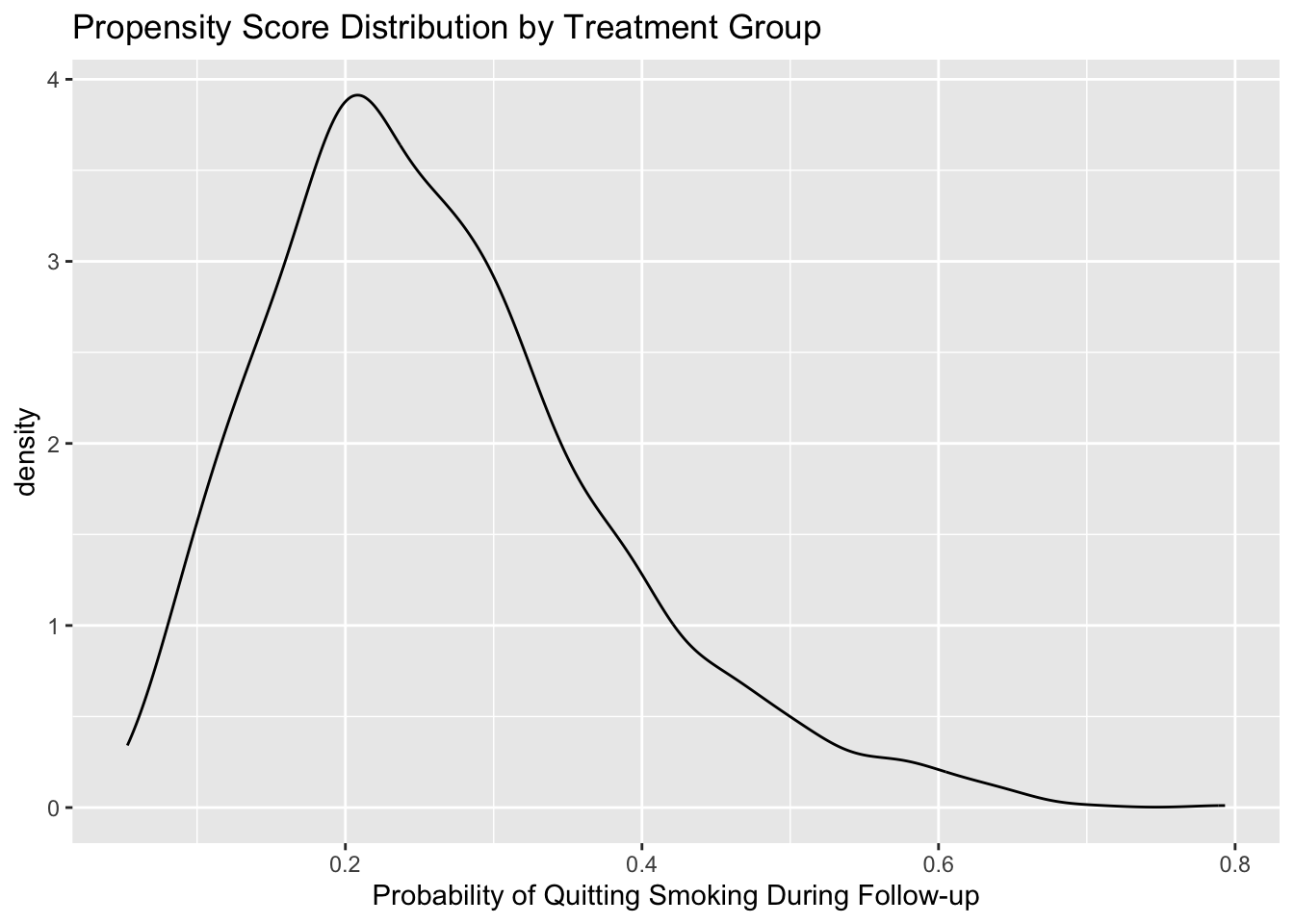
# alternative plot with histograms
ggplot(nhefs, aes(x = ps, fill = as.factor(qsmk), color = as.factor(qsmk))) +
  geom_histogram(alpha = 0.3, position = 'identity', bins=15) +
  facet_grid(as.factor(qsmk) ~ .) +
  xlab('Probability of Quitting Smoking During Follow-up') +
  ggtitle('Propensity Score Distribution by Treatment Group') +
  scale_fill_discrete('') +
  scale_color_discrete('') +
  theme(legend.position = 'bottom', legend.direction = 'vertical')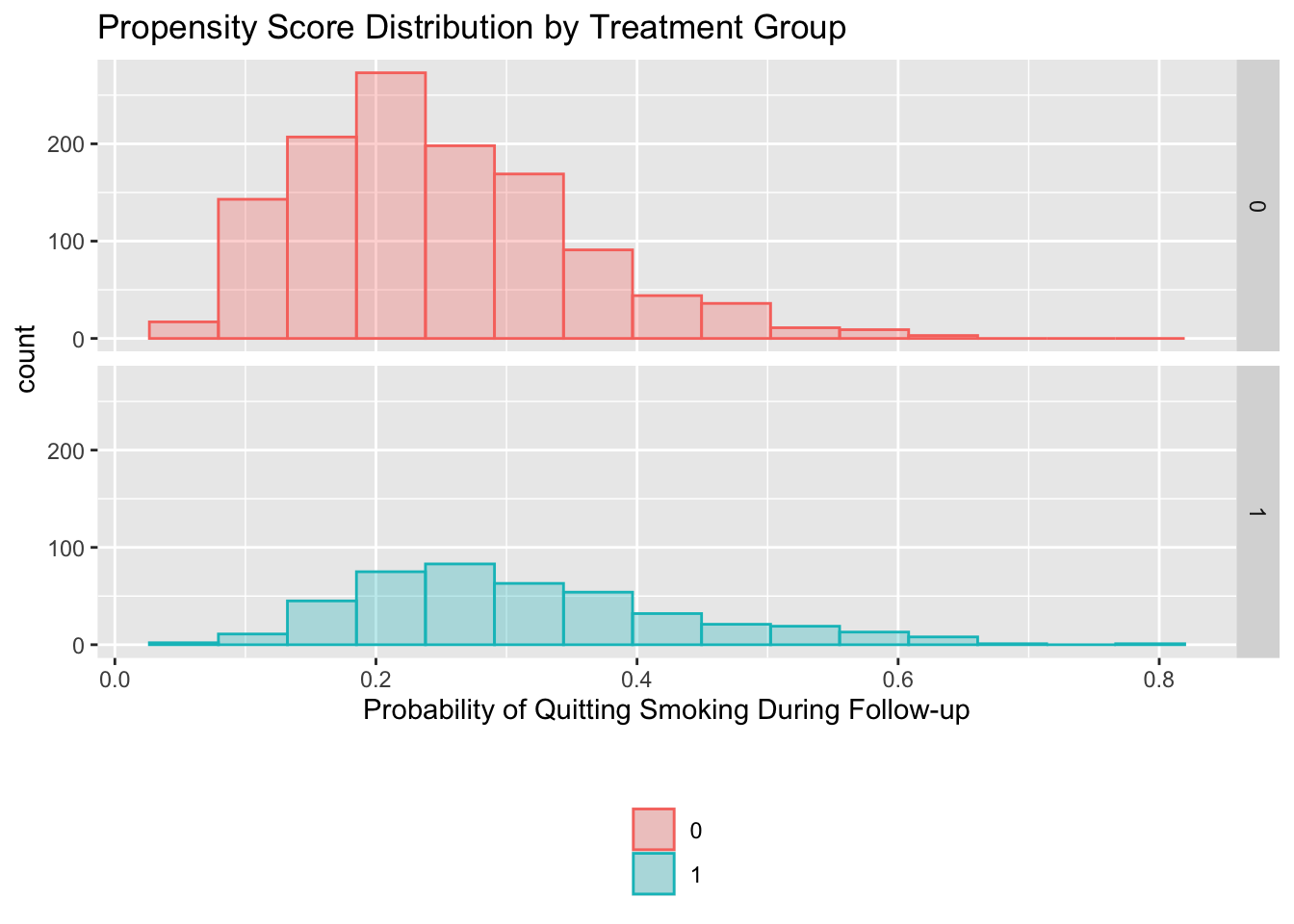
# attempt to reproduce plot from the book
nhefs %>%
  mutate(ps.grp = round(ps/0.05) * 0.05) %>%
  group_by(qsmk, ps.grp) %>%
  summarize(n = n()) %>%
  ungroup() %>%
  mutate(n2 = ifelse(qsmk == 0, yes = n, no =  -1*n)) %>%
  ggplot(aes(x = ps.grp, y = n2, fill = as.factor(qsmk))) +
  geom_bar(stat = 'identity', position = 'identity') +
  geom_text(aes(label = n, x = ps.grp, y = n2 + ifelse(qsmk == 0, 8, -8))) +
  xlab('Probability of Quitting Smoking During Follow-up') +
  ylab('N') +
  ggtitle('Propensity Score Distribution by Treatment Group') +
  scale_fill_discrete('') +
  scale_x_continuous(breaks = seq(0, 1, 0.05)) +
  theme(legend.position = 'bottom', legend.direction = 'vertical',
        axis.ticks.y = element_blank(),
        axis.text.y = element_blank())
Program 15.3
- Stratification on the propensity score
- Data from NHEFS
# calculation of deciles
nhefs$ps.dec <- cut(nhefs$ps,
                    breaks=c(quantile(nhefs$ps, probs=seq(0,1,0.1))),
                    labels=seq(1:10),
                    include.lowest=TRUE)

#install.packages("psych") # install package if required
library("psych")
#>
#> Attaching package: 'psych'
#> The following objects are masked from 'package:ggplot2':
#>
#>     %+%, alpha
describeBy(nhefs$ps, list(nhefs$ps.dec, nhefs$qsmk))
#>
#>  Descriptive statistics by group
#> : 1
#> : 0
#>     vars   n mean    sd median trimmed   mad min max range skew kurtosis   se
#> X1*    1 151   76 43.73     76      76 56.34   1 151   150    0    -1.22 3.56
#> ------------------------------------------------------------
#> : 2
#> : 0
#>     vars   n mean   sd median trimmed   mad min max range skew kurtosis   se
#> X1*    1 136 68.5 39.4   68.5    68.5 50.41   1 136   135    0    -1.23 3.38
#> ------------------------------------------------------------
#> : 3
#> : 0
#>     vars   n mean    sd median trimmed   mad min max range skew kurtosis   se
#> X1*    1 134 67.5 38.83   67.5    67.5 49.67   1 134   133    0    -1.23 3.35
#> ------------------------------------------------------------
#> : 4
#> : 0
#>     vars   n mean    sd median trimmed   mad min max range skew kurtosis   se
#> X1*    1 129   65 37.38     65      65 47.44   1 129   128    0    -1.23 3.29
#> ------------------------------------------------------------
#> : 5
#> : 0
#>     vars   n mean    sd median trimmed   mad min max range skew kurtosis   se
#> X1*    1 120 60.5 34.79   60.5    60.5 44.48   1 120   119    0    -1.23 3.18
#> ------------------------------------------------------------
#> : 6
#> : 0
#>     vars   n mean    sd median trimmed mad min max range skew kurtosis   se
#> X1*    1 117   59 33.92     59      59  43   1 117   116    0    -1.23 3.14
#> ------------------------------------------------------------
#> : 7
#> : 0
#>     vars   n mean    sd median trimmed   mad min max range skew kurtosis   se
#> X1*    1 120 60.5 34.79   60.5    60.5 44.48   1 120   119    0    -1.23 3.18
#> ------------------------------------------------------------
#> : 8
#> : 0
#>     vars   n mean    sd median trimmed   mad min max range skew kurtosis   se
#> X1*    1 112 56.5 32.48   56.5    56.5 41.51   1 112   111    0    -1.23 3.07
#> ------------------------------------------------------------
#> : 9
#> : 0
#>     vars  n mean    sd median trimmed   mad min max range skew kurtosis   se
#> X1*    1 96 48.5 27.86   48.5    48.5 35.58   1  96    95    0    -1.24 2.84
#> ------------------------------------------------------------
#> : 10
#> : 0
#>     vars  n mean    sd median trimmed   mad min max range skew kurtosis   se
#> X1*    1 86 43.5 24.97   43.5    43.5 31.88   1  86    85    0    -1.24 2.69
#> ------------------------------------------------------------
#> : 1
#> : 1
#>     vars  n mean   sd median trimmed  mad min max range skew kurtosis   se
#> X1*    1 12  6.5 3.61    6.5     6.5 4.45   1  12    11    0     -1.5 1.04
#> ------------------------------------------------------------
#> : 2
#> : 1
#>     vars  n mean   sd median trimmed   mad min max range skew kurtosis   se
#> X1*    1 27   14 7.94     14      14 10.38   1  27    26    0    -1.33 1.53
#> ------------------------------------------------------------
#> : 3
#> : 1
#>     vars  n mean   sd median trimmed   mad min max range skew kurtosis   se
#> X1*    1 29   15 8.51     15      15 10.38   1  29    28    0    -1.32 1.58
#> ------------------------------------------------------------
#> : 4
#> : 1
#>     vars  n mean   sd median trimmed  mad min max range skew kurtosis   se
#> X1*    1 34 17.5 9.96   17.5    17.5 12.6   1  34    33    0    -1.31 1.71
#> ------------------------------------------------------------
#> : 5
#> : 1
#>     vars  n mean    sd median trimmed   mad min max range skew kurtosis   se
#> X1*    1 43   22 12.56     22      22 16.31   1  43    42    0    -1.28 1.91
#> ------------------------------------------------------------
#> : 6
#> : 1
#>     vars  n mean    sd median trimmed   mad min max range skew kurtosis   se
#> X1*    1 45   23 13.13     23      23 16.31   1  45    44    0    -1.28 1.96
#> ------------------------------------------------------------
#> : 7
#> : 1
#>     vars  n mean    sd median trimmed   mad min max range skew kurtosis   se
#> X1*    1 43   22 12.56     22      22 16.31   1  43    42    0    -1.28 1.91
#> ------------------------------------------------------------
#> : 8
#> : 1
#>     vars  n mean    sd median trimmed   mad min max range skew kurtosis   se
#> X1*    1 51   26 14.87     26      26 19.27   1  51    50    0    -1.27 2.08
#> ------------------------------------------------------------
#> : 9
#> : 1
#>     vars  n mean    sd median trimmed  mad min max range skew kurtosis   se
#> X1*    1 67   34 19.49     34      34 25.2   1  67    66    0    -1.25 2.38
#> ------------------------------------------------------------
#> : 10
#> : 1
#>     vars  n mean    sd median trimmed   mad min max range skew kurtosis   se
#> X1*    1 77   39 22.37     39      39 28.17   1  77    76    0    -1.25 2.55

# function to create deciles easily
decile <- function(x) {
  return(factor(quantcut(x, seq(0, 1, 0.1), labels = FALSE)))
}

# regression on PS deciles, allowing for effect modification
for (deciles in c(1:10)) {
  print(t.test(wt82_71~qsmk, data=nhefs[which(nhefs$ps.dec==deciles),]))
}
#>
#>  Welch Two Sample t-test
#>
#> data:  wt82_71 by qsmk
#> t = 0.0060506, df = 11.571, p-value = 0.9953
#> alternative hypothesis: true difference in means between group 0 and group 1 is not equal to 0
#> 95 percent confidence interval:
#>  -5.283903  5.313210
#> sample estimates:
#> mean in group 0 mean in group 1
#>        3.995205        3.980551
#>
#>
#>  Welch Two Sample t-test
#>
#> data:  wt82_71 by qsmk
#> t = -3.1117, df = 37.365, p-value = 0.003556
#> alternative hypothesis: true difference in means between group 0 and group 1 is not equal to 0
#> 95 percent confidence interval:
#>  -6.849335 -1.448161
#> sample estimates:
#> mean in group 0 mean in group 1
#>        2.904679        7.053426
#>
#>
#>  Welch Two Sample t-test
#>
#> data:  wt82_71 by qsmk
#> t = -4.5301, df = 35.79, p-value = 6.317e-05
#> alternative hypothesis: true difference in means between group 0 and group 1 is not equal to 0
#> 95 percent confidence interval:
#>  -9.474961 -3.613990
#> sample estimates:
#> mean in group 0 mean in group 1
#>        2.612094        9.156570
#>
#>
#>  Welch Two Sample t-test
#>
#> data:  wt82_71 by qsmk
#> t = -1.4117, df = 45.444, p-value = 0.1648
#> alternative hypothesis: true difference in means between group 0 and group 1 is not equal to 0
#> 95 percent confidence interval:
#>  -5.6831731  0.9985715
#> sample estimates:
#> mean in group 0 mean in group 1
#>        3.474679        5.816979
#>
#>
#>  Welch Two Sample t-test
#>
#> data:  wt82_71 by qsmk
#> t = -3.1371, df = 74.249, p-value = 0.002446
#> alternative hypothesis: true difference in means between group 0 and group 1 is not equal to 0
#> 95 percent confidence interval:
#>  -6.753621 -1.507087
#> sample estimates:
#> mean in group 0 mean in group 1
#>        2.098800        6.229154
#>
#>
#>  Welch Two Sample t-test
#>
#> data:  wt82_71 by qsmk
#> t = -2.1677, df = 50.665, p-value = 0.0349
#> alternative hypothesis: true difference in means between group 0 and group 1 is not equal to 0
#> 95 percent confidence interval:
#>  -8.7516605 -0.3350127
#> sample estimates:
#> mean in group 0 mean in group 1
#>        1.847004        6.390340
#>
#>
#>  Welch Two Sample t-test
#>
#> data:  wt82_71 by qsmk
#> t = -3.3155, df = 84.724, p-value = 0.001348
#> alternative hypothesis: true difference in means between group 0 and group 1 is not equal to 0
#> 95 percent confidence interval:
#>  -6.904207 -1.727590
#> sample estimates:
#> mean in group 0 mean in group 1
#>        1.560048        5.875946
#>
#>
#>  Welch Two Sample t-test
#>
#> data:  wt82_71 by qsmk
#> t = -2.664, df = 75.306, p-value = 0.009441
#> alternative hypothesis: true difference in means between group 0 and group 1 is not equal to 0
#> 95 percent confidence interval:
#>  -6.2396014 -0.9005605
#> sample estimates:
#> mean in group 0 mean in group 1
#>       0.2846851       3.8547661
#>
#>
#>  Welch Two Sample t-test
#>
#> data:  wt82_71 by qsmk
#> t = -1.9122, df = 129.12, p-value = 0.05806
#> alternative hypothesis: true difference in means between group 0 and group 1 is not equal to 0
#> 95 percent confidence interval:
#>  -4.68143608  0.07973698
#> sample estimates:
#> mean in group 0 mean in group 1
#>      -0.8954482       1.4054014
#>
#>
#>  Welch Two Sample t-test
#>
#> data:  wt82_71 by qsmk
#> t = -1.5925, df = 142.72, p-value = 0.1135
#> alternative hypothesis: true difference in means between group 0 and group 1 is not equal to 0
#> 95 percent confidence interval:
#>  -5.0209284  0.5404697
#> sample estimates:
#> mean in group 0 mean in group 1
#>      -0.5043766       1.7358528

# regression on PS deciles, not allowing for effect modification
fit.psdec <- glm(wt82_71 ~ qsmk + as.factor(ps.dec), data = nhefs)
summary(fit.psdec)
#>
#> Call:
#> glm(formula = wt82_71 ~ qsmk + as.factor(ps.dec), data = nhefs)
#>
#> Coefficients:
#>                     Estimate Std. Error t value Pr(>|t|)
#> (Intercept)           3.7505     0.6089   6.159 9.29e-10 ***
#> qsmk                  3.5005     0.4571   7.659 3.28e-14 ***
#> as.factor(ps.dec)2   -0.7391     0.8611  -0.858   0.3908
#> as.factor(ps.dec)3   -0.6182     0.8612  -0.718   0.4730
#> as.factor(ps.dec)4   -0.5204     0.8584  -0.606   0.5444
#> as.factor(ps.dec)5   -1.4884     0.8590  -1.733   0.0834 .
#> as.factor(ps.dec)6   -1.6227     0.8675  -1.871   0.0616 .
#> as.factor(ps.dec)7   -1.9853     0.8681  -2.287   0.0223 *
#> as.factor(ps.dec)8   -3.4447     0.8749  -3.937 8.61e-05 ***
#> as.factor(ps.dec)9   -5.1544     0.8848  -5.825 6.91e-09 ***
#> as.factor(ps.dec)10  -4.8403     0.8828  -5.483 4.87e-08 ***
#> ---
#> Signif. codes:  0 '***' 0.001 '**' 0.01 '*' 0.05 '.' 0.1 ' ' 1
#>
#> (Dispersion parameter for gaussian family taken to be 58.42297)
#>
#>     Null deviance: 97176  on 1565  degrees of freedom
#> Residual deviance: 90848  on 1555  degrees of freedom
#>   (63 observations deleted due to missingness)
#> AIC: 10827
#>
#> Number of Fisher Scoring iterations: 2
confint.lm(fit.psdec)
#>                         2.5 %      97.5 %
#> (Intercept)          2.556098  4.94486263
#> qsmk                 2.603953  4.39700504
#> as.factor(ps.dec)2  -2.428074  0.94982494
#> as.factor(ps.dec)3  -2.307454  1.07103569
#> as.factor(ps.dec)4  -2.204103  1.16333143
#> as.factor(ps.dec)5  -3.173337  0.19657938
#> as.factor(ps.dec)6  -3.324345  0.07893027
#> as.factor(ps.dec)7  -3.688043 -0.28248110
#> as.factor(ps.dec)8  -5.160862 -1.72860113
#> as.factor(ps.dec)9  -6.889923 -3.41883853
#> as.factor(ps.dec)10 -6.571789 -3.10873731
Program 15.4
- Standardization using the propensity score
- Data from NHEFS
#install.packages("boot") # install package if required
library("boot")
#>
#> Attaching package: 'boot'
#> The following object is masked from 'package:psych':
#>
#>     logit
#> The following object is masked from 'package:survival':
#>
#>     aml

# standardization by propensity score, agnostic regarding effect modification
std.ps <- function(data, indices) {
  d <- data[indices,] # 1st copy: equal to original one`
  # calculating propensity scores
  ps.fit <- glm(qsmk ~ sex + race + age + I(age*age)
                + as.factor(education) + smokeintensity
                + I(smokeintensity*smokeintensity) + smokeyrs
                + I(smokeyrs*smokeyrs) + as.factor(exercise)
                + as.factor(active) + wt71 + I(wt71*wt71),
                data=d, family=binomial())
  d$pscore <- predict(ps.fit, d, type="response")

  # create a dataset with 3 copies of each subject
  d$interv <- -1 # 1st copy: equal to original one`
  d0 <- d # 2nd copy: treatment set to 0, outcome to missing
  d0$interv <- 0
  d0$qsmk <- 0
  d0$wt82_71 <- NA
  d1 <- d # 3rd copy: treatment set to 1, outcome to missing
  d1$interv <- 1
  d1$qsmk <- 1
  d1$wt82_71 <- NA
  d.onesample <- rbind(d, d0, d1) # combining datasets

  std.fit <- glm(wt82_71 ~ qsmk + pscore + I(qsmk*pscore), data=d.onesample)
  d.onesample$predicted_meanY <- predict(std.fit, d.onesample)

  # estimate mean outcome in each of the groups interv=-1, interv=0, and interv=1
  return(c(mean(d.onesample$predicted_meanY[d.onesample$interv==-1]),
           mean(d.onesample$predicted_meanY[d.onesample$interv==0]),
           mean(d.onesample$predicted_meanY[d.onesample$interv==1]),
           mean(d.onesample$predicted_meanY[d.onesample$interv==1])-
             mean(d.onesample$predicted_meanY[d.onesample$interv==0])))
}

# bootstrap
results <- boot(data=nhefs, statistic=std.ps, R=5)

# generating confidence intervals
se <- c(sd(results$t[,1]), sd(results$t[,2]),
        sd(results$t[,3]), sd(results$t[,4]))
mean <- results$t0
ll <- mean - qnorm(0.975)*se
ul <- mean + qnorm(0.975)*se

bootstrap <- data.frame(cbind(c("Observed", "No Treatment", "Treatment",
                                "Treatment - No Treatment"), mean, se, ll, ul))
bootstrap
#>                         V1             mean                se               ll
#> 1                 Observed 2.63384609228479 0.221903213692339 2.19892378539411
#> 2             No Treatment 1.71983636149845 0.183362409319646 1.36045264311346
#> 3                Treatment 5.35072300362985 0.352024049657682 4.66076854460886
#> 4 Treatment - No Treatment  3.6308866421314 0.204782650536598 3.22952002242102
#>                 ul
#> 1 3.06876839917547
#> 2 2.07922007988345
#> 3 6.04067746265085
#> 4 4.03225326184178
# regression on the propensity score (linear term)
model6 <- glm(wt82_71 ~ qsmk + ps, data = nhefs) # p.qsmk
summary(model6)
#>
#> Call:
#> glm(formula = wt82_71 ~ qsmk + ps, data = nhefs)
#>
#> Coefficients:
#> Estimate Std. Error t value Pr(>|t|)
#> (Intercept) 5.5945 0.4831 11.581 < 2e-16 ***
#> qsmk 3.5506 0.4573 7.765 1.47e-14 ***
#> ps -14.8218 1.7576 -8.433 < 2e-16 ***
#> ---
#> Signif. codes: 0 '***' 0.001 '**' 0.01 '*' 0.05 '.' 0.1 ' ' 1
#>
#> (Dispersion parameter for gaussian family taken to be 58.28455)
#>
#> Null deviance: 97176 on 1565 degrees of freedom
#> Residual deviance: 91099 on 1563 degrees of freedom
#> (63 observations deleted due to missingness)
#> AIC: 10815
#>
#> Number of Fisher Scoring iterations: 2
# standarization on the propensity score
# (step 1) create two new datasets, one with all treated and one with all untreated
treated <- nhefs
treated$qsmk <- 1
untreated <- nhefs
untreated$qsmk <- 0
# (step 2) predict values for everyone in each new dataset based on above model
treated$pred.y <- predict(model6, treated)
untreated$pred.y <- predict(model6, untreated)
# (step 3) compare mean weight loss had all been treated vs. that had all been untreated
mean1 <- mean(treated$pred.y, na.rm = TRUE)
mean0 <- mean(untreated$pred.y, na.rm = TRUE)
mean1
#> [1] 5.250824
mean0
#> [1] 1.700228
mean1 - mean0
#> [1] 3.550596
# (step 4) bootstrap a confidence interval
# number of bootstraps
nboot <- 100
# set up a matrix to store results
boots <- data.frame(i = 1:nboot,
mean1 = NA,
mean0 = NA,
difference = NA)
# loop to perform the bootstrapping
nhefs <- subset(nhefs, !is.na(ps) & !is.na(wt82_71)) # p.qsmk
for(i in 1:nboot) {
# sample with replacement
sampl <- nhefs[sample(1:nrow(nhefs), nrow(nhefs), replace = TRUE), ]
# fit the model in the bootstrap sample
bootmod <- glm(wt82_71 ~ qsmk + ps, data = sampl) # ps
# create new datasets
sampl.treated <- sampl %>%
mutate(qsmk = 1)
sampl.untreated <- sampl %>%
mutate(qsmk = 0)
# predict values
sampl.treated$pred.y <- predict(bootmod, sampl.treated)
sampl.untreated$pred.y <- predict(bootmod, sampl.untreated)
# output results
boots[i, 'mean1'] <- mean(sampl.treated$pred.y, na.rm = TRUE)
boots[i, 'mean0'] <- mean(sampl.untreated$pred.y, na.rm = TRUE)
boots[i, 'difference'] <- boots[i, 'mean1'] - boots[i, 'mean0']
# once loop is done, print the results
if(i == nboot) {
cat('95% CI for the causal mean difference\n')
cat(mean(boots$difference) - 1.96*sd(boots$difference),
',',
mean(boots$difference) + 1.96*sd(boots$difference))
}
}
#> 95% CI for the causal mean difference
#> 2.529802 , 4.579674A more flexible and elegant way to do this is to write a function to perform the model fitting, prediction, bootstrapping, and reporting all at once.