17. Causal survival analysis: Stata
/***************************************************************
Stata code for Causal Inference: What If by Miguel Hernan & Jamie Robins
Date: 10/10/2019
Author: Eleanor Murray
For errors contact: ejmurray@bu.edu
***************************************************************/
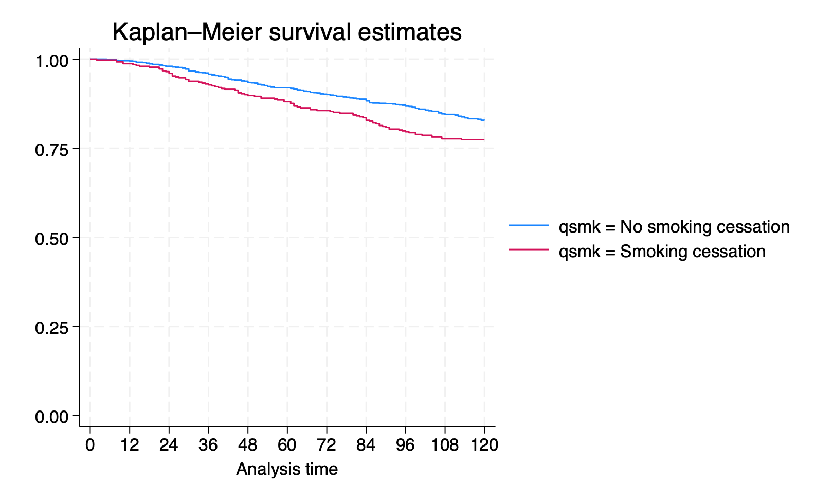
Program 17.1
- Nonparametric estimation of survival curves
- Data from NHEFS
- Section 17.1
use ./data/nhefs-formatted, clear

/*Some preprocessing of the data*/
gen survtime = .
replace survtime = 120 if death == 0
replace survtime = (yrdth - 83)*12 + modth if death ==1
* yrdth ranges from 83 to 92*

tab death qsmk

/*Kaplan-Meier graph of observed survival over time, by quitting smoking*/
*For now, we use the stset function in Stata*
stset survtime, failure(death=1)
sts graph, by(qsmk) xlabel(0(12)120)
qui gr export ./figs/stata-fig-17-1.png, replace
(1,566 missing values generated)

(1,275 real changes made)

(291 real changes made)

     death |
   between | quit smoking between
  1983 and |   baseline and 1982
      1992 | No smokin  Smoking c |     Total
-----------+----------------------+----------
         0 |       963        312 |     1,275
         1 |       200         91 |       291
-----------+----------------------+----------
     Total |     1,163        403 |     1,566


Survival-time data settings

         Failure event: death==1
Observed time interval: (0, survtime]
     Exit on or before: failure

--------------------------------------------------------------------------
      1,566  total observations
          0  exclusions
--------------------------------------------------------------------------
      1,566  observations remaining, representing
        291  failures in single-record/single-failure data
    171,076  total analysis time at risk and under observation
                                                At risk from t =         0
                                     Earliest observed entry t =         0
                                          Last observed exit t =       120

        Failure _d: death==1
  Analysis time _t: survtime
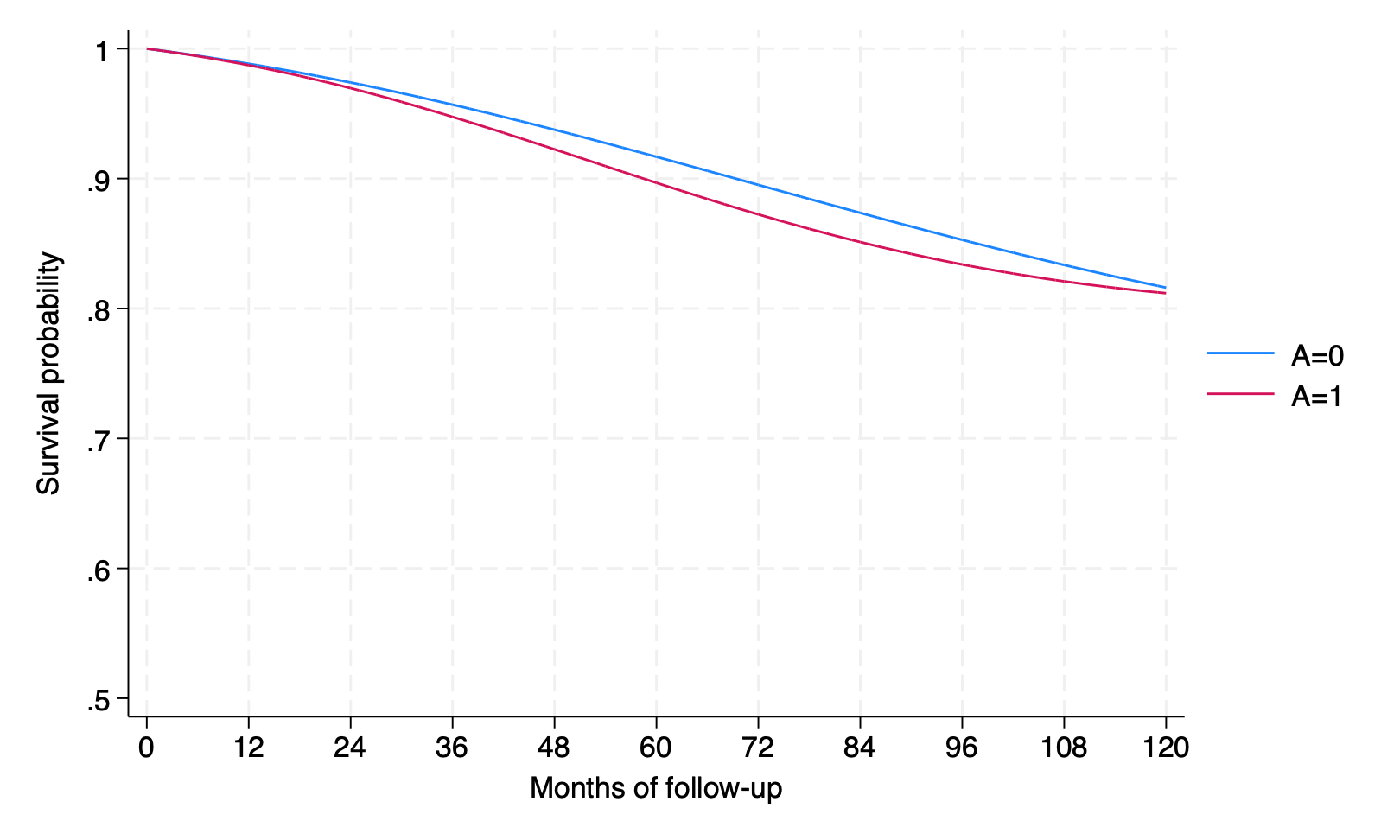
Program 17.2
- Parametric estimation of survival curves via hazards model
- Data from NHEFS
- Section 17.1
- Generates Figure 17.4
/**Create person-month dataset for survival analyses**/

/* We want our new dataset to include 1 observation per person
per month alive, starting at time = 0.
Individuals who survive to the end of follow-up will have
119 time points
Individuals who die will have survtime - 1 time points*/

use ./data/nhefs-formatted, clear

gen survtime = .
replace survtime = 120 if death == 0
replace survtime = (yrdth - 83)*12 + modth if death ==1

*expand data to person-time*
gen time = 0
expand survtime if time == 0
bysort seqn: replace time = _n - 1

*Create event variable*
gen event = 0
replace event = 1 if time == survtime - 1 & death == 1
tab event

*Create time-squared variable for analyses*
gen timesq = time*time

*Save the dataset to your working directory for future use*
qui save ./data/nhefs_surv, replace

/**Hazard ratios**/
use ./data/nhefs_surv, clear

*Fit a pooled logistic hazards model *
logistic event qsmk qsmk#c.time qsmk#c.time#c.time ///
  c.time c.time#c.time

/**Survival curves: run regression then do:**/

*Create a dataset with all time points under each treatment level*
*Re-expand data with rows for all timepoints*
drop if time != 0
expand 120 if time ==0
bysort seqn: replace time = _n - 1

/*Create 2 copies of each subject, and set outcome to missing
and treatment -- use only the newobs*/
expand 2 , generate(interv)
replace qsmk = interv

/*Generate predicted event and survival probabilities
for each person each month in copies*/
predict pevent_k, pr
gen psurv_k = 1-pevent_k
keep seqn time qsmk interv psurv_k

*Within copies, generate predicted survival over time*
*Remember, survival is the product of conditional survival probabilities in each interval*
sort seqn interv time
gen _t = time + 1
gen psurv = psurv_k if _t ==1
bysort seqn interv: replace psurv = psurv_k*psurv[_t-1] if _t >1

*Display 10-year standardized survival, under interventions*
*Note: since time starts at 0, month 119 is 10-year survival*
by interv, sort: summarize psurv if time == 119

*Graph of standardized survival over time, under interventions*
/*Note, we want our graph to start at 100% survival,
so add an extra time point with P(surv) = 1*/
expand 2 if time ==0, generate(newtime)
replace psurv  = 1 if newtime == 1
gen time2 = 0 if newtime ==1
replace time2 = time + 1 if newtime == 0

/*Separate the survival probabilities to allow plotting by
intervention on qsmk*/
separate psurv, by(interv)

*Plot the curves*
twoway (line psurv0 time2, sort) ///
  (line psurv1 time2, sort) if interv > -1 ///
  , ylabel(0.5(0.1)1.0) xlabel(0(12)120) ///
  ytitle("Survival probability") xtitle("Months of follow-up") ///
  legend(label(1 "A=0") label(2 "A=1"))
qui gr export ./figs/stata-fig-17-2.png, replace
(1,566 missing values generated)

(1,275 real changes made)

(291 real changes made)


(169,510 observations created)

(169510 real changes made)


(291 real changes made)

      event |      Freq.     Percent        Cum.
------------+-----------------------------------
          0 |    170,785       99.83       99.83
          1 |        291        0.17      100.00
------------+-----------------------------------
      Total |    171,076      100.00


Logistic regression                                    Number of obs = 171,076
                                                       LR chi2(5)    =   24.26
                                                       Prob > chi2   =  0.0002
Log likelihood = -2134.1973                            Pseudo R2     =  0.0057

------------------------------------------------------------------------------------
             event | Odds ratio   Std. err.      z    P>|z|     [95% conf. interval]
-------------------+----------------------------------------------------------------
              qsmk |   1.402527   .6000025     0.79   0.429     .6064099    3.243815
                   |
       qsmk#c.time |
Smoking cessation  |   1.012318   .0162153     0.76   0.445     .9810299    1.044603
                   |
qsmk#c.time#c.time |
Smoking cessation  |   .9998342   .0001321    -1.25   0.210     .9995753    1.000093
                   |
              time |   1.022048   .0090651     2.46   0.014     1.004434    1.039971
                   |
     c.time#c.time |   .9998637   .0000699    -1.95   0.051     .9997266    1.000001
                   |
             _cons |   .0007992   .0001972   -28.90   0.000     .0004927    .0012963
------------------------------------------------------------------------------------
Note: _cons estimates baseline odds.

(169,510 observations deleted)

(186,354 observations created)

(186354 real changes made)

(187,920 observations created)

(187,920 real changes made)


(372,708 missing values generated)

(372708 real changes made)


--------------------------------------------------------------------------------------
-> interv = Original

    Variable |        Obs        Mean    Std. dev.       Min        Max
-------------+---------------------------------------------------------
       psurv |      1,566    .8279829           0   .8279829   .8279829

--------------------------------------------------------------------------------------
-> interv = Duplicat

    Variable |        Obs        Mean    Std. dev.       Min        Max
-------------+---------------------------------------------------------
       psurv |      1,566     .774282           0    .774282    .774282


(3,132 observations created)

(3,132 real changes made)

(375,840 missing values generated)

(375,840 real changes made)


Variable      Storage   Display    Value
    name         type    format    label      Variable label
--------------------------------------------------------------------------------------
psurv0          float   %9.0g                 psurv, interv == Original observation
psurv1          float   %9.0g                 psurv, interv == Duplicated observation
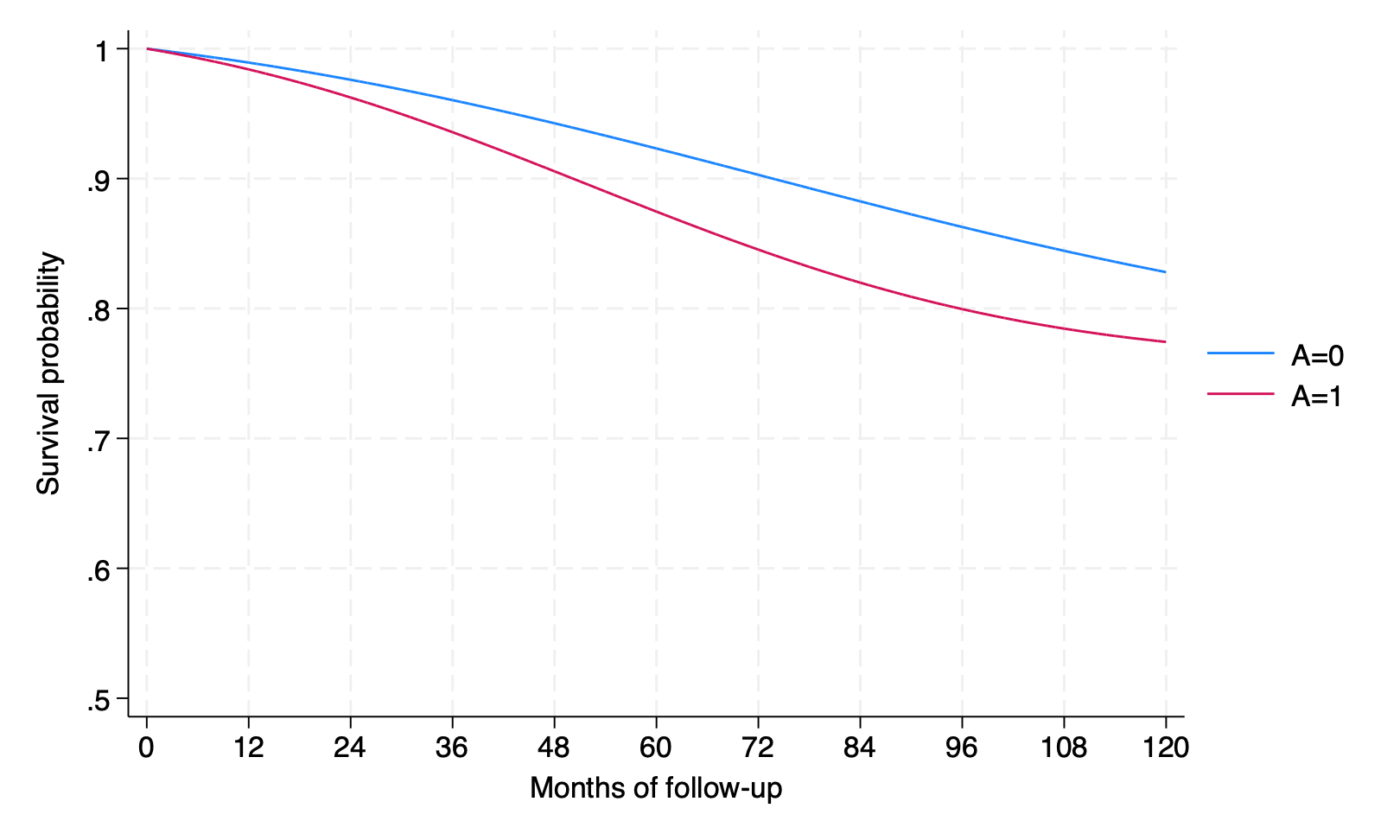
Program 17.3
- Estimation of survival curves via IP weighted hazards model
- Data from NHEFS
- Section 17.4
- Generates Figure 17.6
use ./data/nhefs_surv, clear

keep seqn event qsmk time sex race age education ///
  smokeintensity smkintensity82_71 smokeyrs ///
  exercise active wt71
preserve

*Estimate weights*
logit qsmk sex race c.age##c.age ib(last).education ///
  c.smokeintensity##c.smokeintensity ///
  c.smokeyrs##c.smokeyrs ib(last).exercise ///
  ib(last).active c.wt71##c.wt71 if time == 0
predict p_qsmk, pr

logit qsmk if time ==0
predict num, pr
gen sw=num/p_qsmk if qsmk==1
replace sw=(1-num)/(1-p_qsmk) if qsmk==0
summarize sw

*IP weighted survival by smoking cessation*
logit event qsmk qsmk#c.time qsmk#c.time#c.time ///
  c.time c.time#c.time [pweight=sw] , cluster(seqn)

*Create a dataset with all time points under each treatment level*
*Re-expand data with rows for all timepoints*
drop if time != 0
expand 120 if time ==0
bysort seqn: replace time = _n - 1

/*Create 2 copies of each subject, and set outcome
to missing and treatment -- use only the newobs*/
expand 2 , generate(interv)
replace qsmk = interv

/*Generate predicted event and survival probabilities
for each person each month in copies*/
predict pevent_k, pr
gen psurv_k = 1-pevent_k
keep seqn time qsmk interv psurv_k

*Within copies, generate predicted survival over time*
/*Remember, survival is the product of conditional survival
probabilities in each interval*/
sort seqn interv time
gen _t = time + 1
gen psurv = psurv_k if _t ==1
bysort seqn interv: replace psurv = psurv_k*psurv[_t-1] if _t >1

*Display 10-year standardized survival, under interventions*
*Note: since time starts at 0, month 119 is 10-year survival*
by interv, sort: summarize psurv if time == 119

quietly summarize psurv if(interv==0 & time ==119)
matrix input observe = (0,`r(mean)')
quietly summarize psurv if(interv==1 & time ==119)
matrix observe = (observe \1,`r(mean)')
matrix observe = (observe \3, observe[2,2]-observe[1,2])
matrix list observe

*Graph of standardized survival over time, under interventions*
/*Note: since our outcome model has no covariates,
we can plot psurv directly.
If we had covariates we would need to stratify or average across the values*/
expand 2 if time ==0, generate(newtime)
replace psurv  = 1 if newtime == 1
gen time2 = 0 if newtime ==1
replace time2 = time + 1 if newtime == 0
separate psurv, by(interv)
twoway (line psurv0 time2, sort) ///
  (line psurv1 time2, sort) if interv > -1 ///
  , ylabel(0.5(0.1)1.0) xlabel(0(12)120) ///
  ytitle("Survival probability") xtitle("Months of follow-up") ///
  legend(label(1 "A=0") label(2 "A=1"))
qui gr export ./figs/stata-fig-17-3.png, replace

*remove extra timepoint*
drop if newtime == 1
drop time2

restore

**Bootstraps**
qui save ./data/nhefs_std1 , replace

capture program drop bootipw_surv

program define bootipw_surv , rclass
use ./data/nhefs_std1 , clear
preserve
bsample, cluster(seqn) idcluster(newseqn)

logit qsmk sex race c.age##c.age ib(last).education ///
  c.smokeintensity##c.smokeintensity ///
    c.smokeyrs##c.smokeyrs ib(last).exercise ib(last).active ///
    c.wt71##c.wt71 if time == 0
predict p_qsmk, pr

logit qsmk if time ==0
predict num, pr

gen sw=num/p_qsmk if qsmk==1
replace sw=(1-num)/(1-p_qsmk) if qsmk==0

logit event qsmk qsmk#c.time qsmk#c.time#c.time ///
  c.time c.time#c.time [pweight=sw], cluster(newseqn)

drop if time != 0
expand 120 if time ==0
bysort newseqn: replace time = _n - 1
expand 2 , generate(interv_b)
replace qsmk = interv_b

predict pevent_k, pr
gen psurv_k = 1-pevent_k
keep newseqn time qsmk interv_b psurv_k

sort newseqn interv_b time
gen _t = time + 1
gen psurv = psurv_k if _t ==1
bysort newseqn interv_b: ///
  replace psurv = psurv_k*psurv[_t-1] if _t >1
drop if time != 119
bysort interv_b: egen meanS_b = mean(psurv)
keep newseqn qsmk  meanS_b
drop if newseqn != 1  /* only need one pair */

drop newseqn

return scalar boot_0 = meanS_b[1]
return scalar boot_1 = meanS_b[2]
return scalar  boot_diff = return(boot_1) - return(boot_0)
restore
end

set rmsg on
simulate PrY_a0 = r(boot_0) PrY_a1 = r(boot_1) ///
  difference=r(boot_diff), reps(10) seed(1): bootipw_surv
set rmsg off

matrix pe = observe[1..3, 2]'
bstat, stat(pe) n(1629)
Iteration 0:  Log likelihood = -893.02712
Iteration 1:  Log likelihood = -839.70016
Iteration 2:  Log likelihood = -838.45045
Iteration 3:  Log likelihood = -838.44842
Iteration 4:  Log likelihood = -838.44842

Logistic regression                                     Number of obs =  1,566
                                                        LR chi2(18)   = 109.16
                                                        Prob > chi2   = 0.0000
Log likelihood = -838.44842                             Pseudo R2     = 0.0611

-----------------------------------------------------------------------------------
             qsmk | Coefficient  Std. err.      z    P>|z|     [95% conf. interval]
------------------+----------------------------------------------------------------
              sex |  -.5274782   .1540497    -3.42   0.001      -.82941   -.2255463
             race |  -.8392636   .2100668    -4.00   0.000    -1.250987   -.4275404
              age |   .1212052   .0512663     2.36   0.018     .0207251    .2216853
                  |
      c.age#c.age |  -.0008246   .0005361    -1.54   0.124    -.0018753    .0002262
                  |
        education |
               1  |  -.4759606   .2262238    -2.10   0.035    -.9193511   -.0325701
               2  |  -.5047361    .217597    -2.32   0.020    -.9312184   -.0782538
               3  |  -.3895288   .1914353    -2.03   0.042    -.7647351   -.0143226
               4  |  -.4123596   .2772868    -1.49   0.137    -.9558318    .1311126
                  |
   smokeintensity |  -.0772704   .0152499    -5.07   0.000    -.1071596   -.0473812
                  |
 c.smokeintensity#|
 c.smokeintensity |   .0010451   .0002866     3.65   0.000     .0004835    .0016068
                  |
         smokeyrs |  -.0735966   .0277775    -2.65   0.008    -.1280395   -.0191538
                  |
       c.smokeyrs#|
       c.smokeyrs |   .0008441   .0004632     1.82   0.068    -.0000637    .0017519
                  |
         exercise |
               0  |   -.395704   .1872401    -2.11   0.035    -.7626878   -.0287201
               1  |  -.0408635   .1382674    -0.30   0.768    -.3118627    .2301357
                  |
           active |
               0  |   -.176784   .2149721    -0.82   0.411    -.5981215    .2445535
               1  |  -.1448395   .2111472    -0.69   0.493    -.5586806    .2690015
                  |
             wt71 |  -.0152357   .0263161    -0.58   0.563    -.0668144     .036343
                  |
    c.wt71#c.wt71 |   .0001352   .0001632     0.83   0.407    -.0001846     .000455
                  |
            _cons |   -1.19407   1.398493    -0.85   0.393    -3.935066    1.546925
-----------------------------------------------------------------------------------


Iteration 0:  Log likelihood = -893.02712
Iteration 1:  Log likelihood = -893.02712

Logistic regression                                    Number of obs =   1,566
                                                       LR chi2(0)    =   -0.00
                                                       Prob > chi2   =       .
Log likelihood = -893.02712                            Pseudo R2     = -0.0000

------------------------------------------------------------------------------
        qsmk | Coefficient  Std. err.      z    P>|z|     [95% conf. interval]
-------------+----------------------------------------------------------------
       _cons |  -1.059822   .0578034   -18.33   0.000    -1.173114    -.946529
------------------------------------------------------------------------------


(128,481 missing values generated)

(128,481 real changes made)

    Variable |        Obs        Mean    Std. dev.       Min        Max
-------------+---------------------------------------------------------
          sw |    171,076    1.000509    .2851505   .3312489   4.297662


Iteration 0:  Log pseudolikelihood = -2136.3671
Iteration 1:  Log pseudolikelihood = -2127.0974
Iteration 2:  Log pseudolikelihood = -2126.8556
Iteration 3:  Log pseudolikelihood = -2126.8554

Logistic regression                                    Number of obs = 171,076
                                                       Wald chi2(5)  =   22.74
                                                       Prob > chi2   =  0.0004
Log pseudolikelihood = -2126.8554                      Pseudo R2     =  0.0045

                                     (Std. err. adjusted for 1,566 clusters in seqn)
------------------------------------------------------------------------------------
                   |               Robust
             event | Coefficient  std. err.      z    P>|z|     [95% conf. interval]
-------------------+----------------------------------------------------------------
              qsmk |  -.1301273   .4186673    -0.31   0.756    -.9507002    .6904456
                   |
       qsmk#c.time |
Smoking cessation  |     .01916   .0151318     1.27   0.205    -.0104978    .0488178
                   |
qsmk#c.time#c.time |
Smoking cessation  |  -.0002152   .0001213    -1.77   0.076    -.0004528    .0000225
                   |
              time |   .0208179   .0077769     2.68   0.007     .0055754    .0360604
                   |
     c.time#c.time |  -.0001278   .0000643    -1.99   0.047    -.0002537   -1.84e-06
                   |
             _cons |  -7.038847   .2142855   -32.85   0.000    -7.458839   -6.618855
------------------------------------------------------------------------------------

(169,510 observations deleted)

(186,354 observations created)

(186354 real changes made)

(187,920 observations created)

(187,920 real changes made)


(372,708 missing values generated)

(372708 real changes made)


--------------------------------------------------------------------------------------
-> interv = Original

    Variable |        Obs        Mean    Std. dev.       Min        Max
-------------+---------------------------------------------------------
       psurv |      1,566    .8161003           0   .8161003   .8161003

--------------------------------------------------------------------------------------
-> interv = Duplicat

    Variable |        Obs        Mean    Std. dev.       Min        Max
-------------+---------------------------------------------------------
       psurv |      1,566    .8116784           0   .8116784   .8116784


observe[3,2]
            c1          c2
r1           0    .8161003
r2           1   .81167841
r3           3  -.00442189

(3,132 observations created)

(3,132 real changes made)

(375,840 missing values generated)

(375,840 real changes made)


Variable      Storage   Display    Value
    name         type    format    label      Variable label
--------------------------------------------------------------------------------------
psurv0          float   %9.0g                 psurv, interv == Original observation
psurv1          float   %9.0g                 psurv, interv == Duplicated observation


(3,132 observations deleted)


  5. predict p_qsmk, pr
  6.
 11.
 23. drop if time != 119
 24. bysort interv_b: egen meanS_b = mean(psurv)
 25. keep newseqn qsmk  meanS_b
 26. drop if newseqn != 1  /* only need one pair */
 27.

r; t=0.00 11:54:12

      Command: bootipw_surv
       PrY_a0: r(boot_0)
       PrY_a1: r(boot_1)
   difference: r(boot_diff)

Simulations (10): .........10 done
r; t=21.24 11:54:33


Bootstrap results                                        Number of obs = 1,629
                                                         Replications  =    10

------------------------------------------------------------------------------
             |   Observed   Bootstrap                         Normal-based
             | coefficient  std. err.      z    P>|z|     [95% conf. interval]
-------------+----------------------------------------------------------------
      PrY_a0 |   .8161003   .0093124    87.64   0.000     .7978484    .8343522
      PrY_a1 |   .8116784   .0237581    34.16   0.000     .7651133    .8582435
  difference |  -.0044219   .0225007    -0.20   0.844    -.0485224    .0396786
------------------------------------------------------------------------------
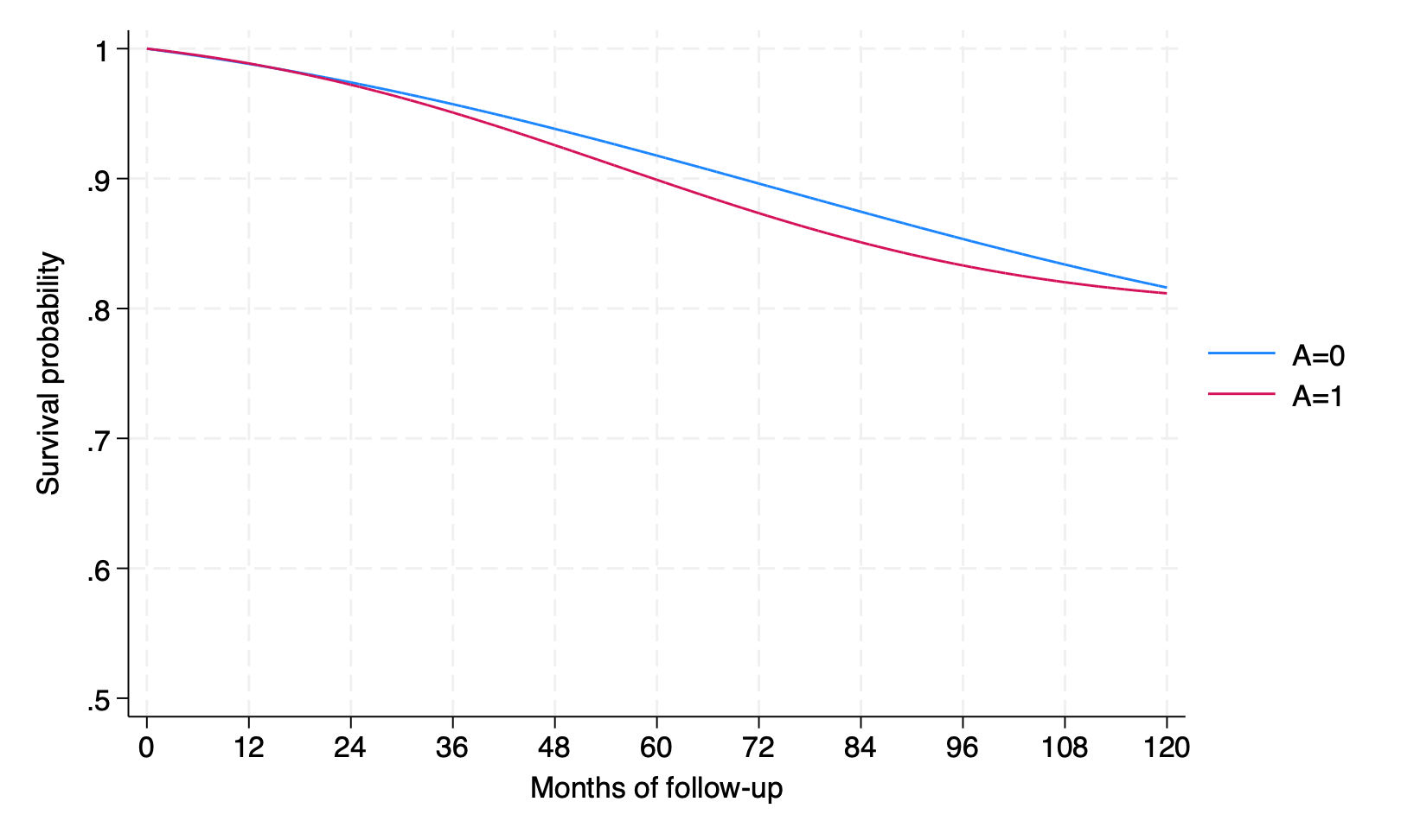
Program 17.4
- Estimating of survival curves via g-formula
- Data from NHEFS
- Section 17.5
- Generates Figure 17.7
use ./data/nhefs_surv, clear

keep seqn event qsmk time sex race age education ///
  smokeintensity smkintensity82_71  smokeyrs exercise ///
  active wt71
preserve

quietly logistic event qsmk qsmk#c.time ///
  qsmk#c.time#c.time time c.time#c.time  ///
    sex race c.age##c.age ib(last).education ///
    c.smokeintensity##c.smokeintensity ///
    c.smokeyrs##c.smokeyrs ib(last).exercise ib(last).active ///
    c.wt71##c.wt71 , cluster(seqn)

drop if time != 0
expand 120 if time ==0
bysort seqn: replace time = _n - 1
expand 2 , generate(interv)
replace qsmk = interv
predict pevent_k, pr
gen psurv_k = 1-pevent_k
keep seqn  time qsmk interv psurv_k
sort seqn interv time
gen _t = time + 1
gen psurv = psurv_k if _t ==1
bysort seqn interv: replace psurv = psurv_k*psurv[_t-1] if _t >1
by interv, sort: summarize psurv if time == 119

keep qsmk interv psurv time

bysort interv : egen meanS = mean(psurv) if time == 119
by interv: summarize meanS

quietly summarize meanS if(qsmk==0  & time ==119)
matrix input observe = ( 0,`r(mean)')
quietly summarize meanS if(qsmk==1  & time ==119)
matrix observe = (observe \1,`r(mean)')
matrix observe = (observe \2, observe[2,2]-observe[1,2])
*Add some row/column descriptions and print results to screen*
matrix rownames observe =  P(Y(a=0)=1) P(Y(a=1)=1) difference
matrix colnames observe = interv survival

*Graph standardized survival over time, under interventions*
/*Note: unlike in Program 17.3, we now have covariates
so we first need to average survival across strata*/
bysort interv time : egen meanS_t = mean(psurv)

*Now we can continue with the graph*
expand 2 if time ==0, generate(newtime)
replace meanS_t  = 1 if newtime == 1
gen time2 = 0 if newtime ==1
replace time2 = time + 1 if newtime == 0
separate meanS_t, by(interv)

twoway (line meanS_t0 time2, sort) ///
  (line meanS_t1 time2, sort) ///
  , ylabel(0.5(0.1)1.0) xlabel(0(12)120) ///
  ytitle("Survival probability") xtitle("Months of follow-up") ///
  legend(label(1 "A=0") label(2 "A=1"))
gr export ./figs/stata-fig-17-4.png, replace

*remove extra timepoint*
drop if newtime == 1

restore

*Bootstraps*
qui save ./data/nhefs_std2 , replace

capture program drop bootstdz_surv

program define bootstdz_surv , rclass
use ./data/nhefs_std2 , clear
preserve

bsample, cluster(seqn) idcluster(newseqn)
logistic event qsmk qsmk#c.time qsmk#c.time#c.time ///
  time c.time#c.time ///
    sex race c.age##c.age ib(last).education ///
    c.smokeintensity##c.smokeintensity c.smkintensity82_71 ///
    c.smokeyrs##c.smokeyrs ib(last).exercise ib(last).active ///
    c.wt71##c.wt71
drop if time != 0
/*only predict on new version of data */
expand 120 if time ==0
bysort newseqn: replace time = _n - 1
expand 2 , generate(interv_b)
replace qsmk = interv_b
predict pevent_k, pr
gen psurv_k = 1-pevent_k
keep newseqn  time qsmk psurv_k
sort newseqn qsmk time
gen _t = time + 1
gen psurv = psurv_k if _t ==1
bysort newseqn  qsmk: replace psurv = psurv_k*psurv[_t-1] if _t >1
drop  if time != 119   /* keep only last observation */
keep newseqn qsmk psurv
/* if time is in data for complete graph add time to bysort */
bysort qsmk  : egen meanS_b = mean(psurv)
keep newseqn qsmk  meanS_b
drop if newseqn != 1  /* only need one pair */
drop newseqn

return scalar boot_0 = meanS_b[1]
return scalar boot_1 = meanS_b[2]
return scalar boot_diff = return(boot_1) - return(boot_0)
restore
end

set rmsg on
simulate PrY_a0 = r(boot_0) PrY_a1 = r(boot_1) ///
  difference=r(boot_diff), reps(10) seed(1): bootstdz_surv
set rmsg off

matrix pe = observe[1..3, 2]'
bstat, stat(pe) n(1629)
(169,510 observations deleted)

(186,354 observations created)

(186354 real changes made)

(187,920 observations created)

(187,920 real changes made)


(372,708 missing values generated)

(372708 real changes made)


--------------------------------------------------------------------------------------
-> interv = Original

    Variable |        Obs        Mean    Std. dev.       Min        Max
-------------+---------------------------------------------------------
       psurv |      1,566    .8160697    .2014345    .014127   .9903372

--------------------------------------------------------------------------------------
-> interv = Duplicat

    Variable |        Obs        Mean    Std. dev.       Min        Max
-------------+---------------------------------------------------------
       psurv |      1,566     .811763    .2044758   .0123403   .9900259


(372,708 missing values generated)


--------------------------------------------------------------------------------------
-> interv = Original

    Variable |        Obs        Mean    Std. dev.       Min        Max
-------------+---------------------------------------------------------
       meanS |      1,566    .8160697           0   .8160697   .8160697

--------------------------------------------------------------------------------------
-> interv = Duplicat

    Variable |        Obs        Mean    Std. dev.       Min        Max
-------------+---------------------------------------------------------
       meanS |      1,566    .8117629           0   .8117629   .8117629


(3,132 observations created)

(3,132 real changes made)

(375,840 missing values generated)

(375,840 real changes made)


Variable      Storage   Display    Value
    name         type    format    label      Variable label
--------------------------------------------------------------------------------------
meanS_t0        float   %9.0g                 meanS_t, interv == Original observation
meanS_t1        float   %9.0g                 meanS_t, interv == Duplicated
                                                observation


file /Users/eptmp/Documents/GitHub/cibookex-r/figs/stata-fig-17-4.png saved as PNG
    format

(3,132 observations deleted)


  5. drop if time != 0
  6. /*only predict on new version of data */

r; t=0.00 11:54:40

      Command: bootstdz_surv
       PrY_a0: r(boot_0)
       PrY_a1: r(boot_1)
   difference: r(boot_diff)

Simulations (10): .........10 done
r; t=22.88 11:55:03


Bootstrap results                                        Number of obs = 1,629
                                                         Replications  =    10

------------------------------------------------------------------------------
             |   Observed   Bootstrap                         Normal-based
             | coefficient  std. err.      z    P>|z|     [95% conf. interval]
-------------+----------------------------------------------------------------
      PrY_a0 |   .8160697   .0087193    93.59   0.000     .7989802    .8331593
      PrY_a1 |   .8117629   .0292177    27.78   0.000     .7544973    .8690286
  difference |  -.0043068   .0307674    -0.14   0.889    -.0646099    .0559963
------------------------------------------------------------------------------