17. Causal survival analysis
Program 17.1
- Nonparametric estimation of survival curves
- Data from NHEFS
library("readxl")
nhefs <- read_excel(here("data","NHEFS.xls"))

# some preprocessing of the data
nhefs$survtime <- ifelse(nhefs$death==0, 120,
                         (nhefs$yrdth-83)*12+nhefs$modth) # yrdth ranges from 83 to 92

table(nhefs$death, nhefs$qsmk)
#>
#>       0   1
#>   0 985 326
#>   1 216 102
summary(nhefs[which(nhefs$death==1),]$survtime)
#>    Min. 1st Qu.  Median    Mean 3rd Qu.    Max.
#>    1.00   35.00   61.00   61.14   86.75  120.00

#install.packages("survival")
#install.packages("ggplot2") # for plots
#install.packages("survminer") # for plots
library("survival")
library("ggplot2")
library("survminer")
#> Loading required package: ggpubr
#>
#> Attaching package: 'survminer'
#> The following object is masked from 'package:survival':
#>
#>     myeloma
survdiff(Surv(survtime, death) ~ qsmk, data=nhefs)
#> Call:
#> survdiff(formula = Surv(survtime, death) ~ qsmk, data = nhefs)
#>
#>           N Observed Expected (O-E)^2/E (O-E)^2/V
#> qsmk=0 1201      216    237.5      1.95      7.73
#> qsmk=1  428      102     80.5      5.76      7.73
#>
#>  Chisq= 7.7  on 1 degrees of freedom, p= 0.005

fit <- survfit(Surv(survtime, death) ~ qsmk, data=nhefs)
ggsurvplot(fit, data = nhefs, xlab="Months of follow-up",
           ylab="Survival probability",
           title="Product-Limit Survival Estimates", risk.table = TRUE,
           fontsize = 3)
#> Ignoring unknown labels:
#> • colour : "Strata"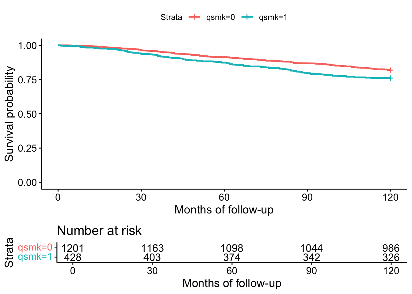
Program 17.2
- Parametric estimation of survival curves via hazards model
- Data from NHEFS
# creation of person-month data
#install.packages("splitstackshape")
library("splitstackshape")
nhefs.surv <- expandRows(nhefs, "survtime", drop=F)
nhefs.surv$time <- sequence(rle(nhefs.surv$seqn)$lengths)-1
nhefs.surv$event <- ifelse(nhefs.surv$time==nhefs.surv$survtime-1 &
                             nhefs.surv$death==1, 1, 0)
nhefs.surv$timesq <- nhefs.surv$time^2

# fit of parametric hazards model
hazards.model <- glm(event==0 ~ qsmk + I(qsmk*time) + I(qsmk*timesq) +
                       time + timesq, family=binomial(), data=nhefs.surv)
summary(hazards.model)
#>
#> Call:
#> glm(formula = event == 0 ~ qsmk + I(qsmk * time) + I(qsmk * timesq) +
#>     time + timesq, family = binomial(), data = nhefs.surv)
#>
#> Coefficients:
#>                    Estimate Std. Error z value Pr(>|z|)
#> (Intercept)       6.996e+00  2.309e-01  30.292   <2e-16 ***
#> qsmk             -3.355e-01  3.970e-01  -0.845   0.3981
#> I(qsmk * time)   -1.208e-02  1.503e-02  -0.804   0.4215
#> I(qsmk * timesq)  1.612e-04  1.246e-04   1.293   0.1960
#> time             -1.960e-02  8.413e-03  -2.329   0.0198 *
#> timesq            1.256e-04  6.686e-05   1.878   0.0604 .
#> ---
#> Signif. codes:  0 '***' 0.001 '**' 0.01 '*' 0.05 '.' 0.1 ' ' 1
#>
#> (Dispersion parameter for binomial family taken to be 1)
#>
#>     Null deviance: 4655.3  on 176763  degrees of freedom
#> Residual deviance: 4631.3  on 176758  degrees of freedom
#> AIC: 4643.3
#>
#> Number of Fisher Scoring iterations: 9

# creation of dataset with all time points under each treatment level
qsmk0 <- data.frame(cbind(seq(0, 119),0,(seq(0, 119))^2))
qsmk1 <- data.frame(cbind(seq(0, 119),1,(seq(0, 119))^2))

colnames(qsmk0) <- c("time", "qsmk", "timesq")
colnames(qsmk1) <- c("time", "qsmk", "timesq")

# assignment of estimated (1-hazard) to each person-month */
qsmk0$p.noevent0 <- predict(hazards.model, qsmk0, type="response")
qsmk1$p.noevent1 <- predict(hazards.model, qsmk1, type="response")

# computation of survival for each person-month
qsmk0$surv0 <- cumprod(qsmk0$p.noevent0)
qsmk1$surv1 <- cumprod(qsmk1$p.noevent1)

# some data management to plot estimated survival curves
hazards.graph <- merge(qsmk0, qsmk1, by=c("time", "timesq"))
hazards.graph$survdiff <- hazards.graph$surv1-hazards.graph$surv0

# plot
ggplot(hazards.graph, aes(x=time, y=surv)) +
  geom_line(aes(y = surv0, colour = "0")) +
  geom_line(aes(y = surv1, colour = "1")) +
  xlab("Months") +
  scale_x_continuous(limits = c(0, 120), breaks=seq(0,120,12)) +
  scale_y_continuous(limits=c(0.6, 1), breaks=seq(0.6, 1, 0.2)) +
  ylab("Survival") +
  ggtitle("Survival from hazards model") +
  labs(colour="A:") +
  theme_bw() +
  theme(legend.position="bottom")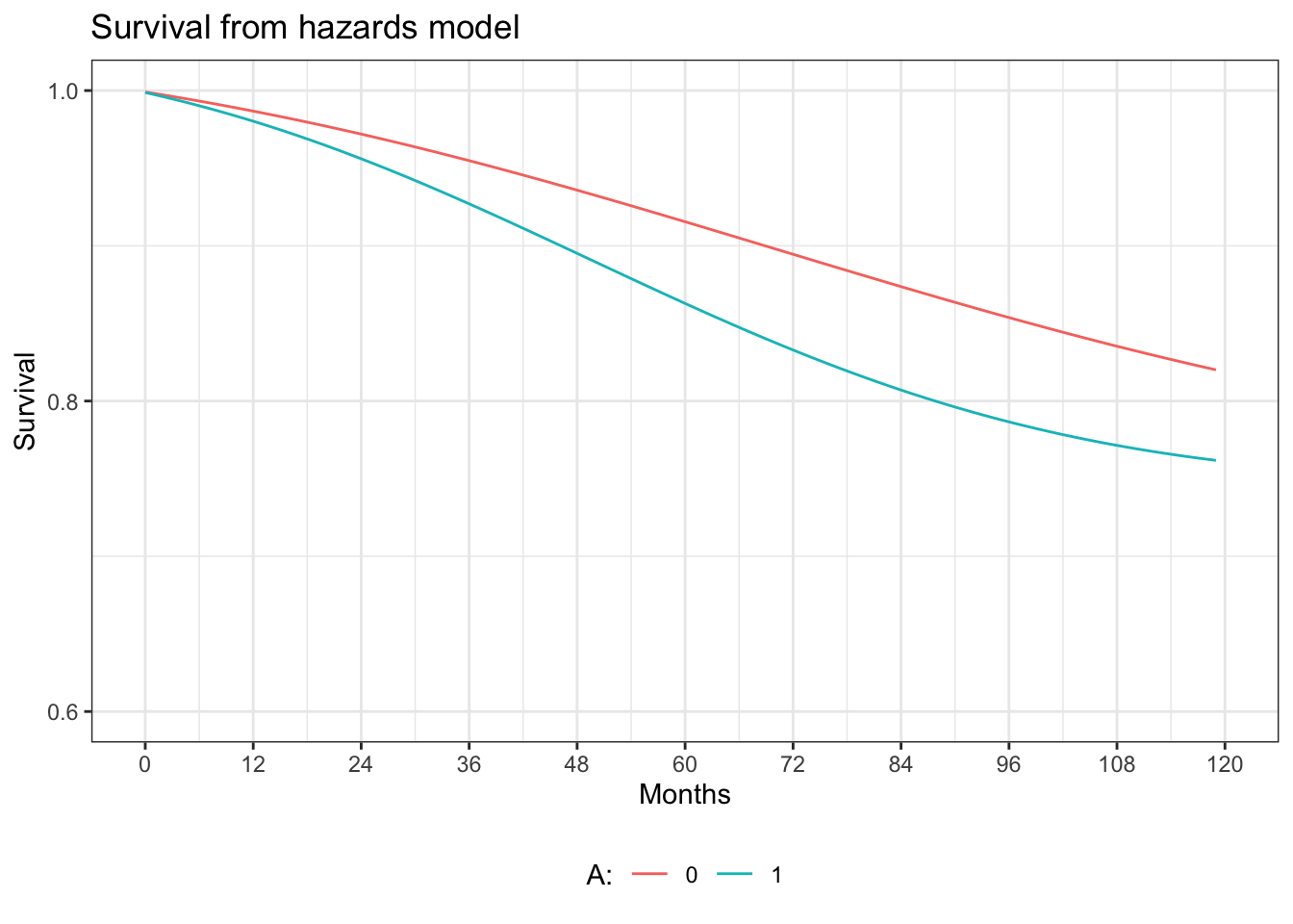
Program 17.3
- Estimation of survival curves via IP weighted hazards model
- Data from NHEFS
# estimation of denominator of ip weights
p.denom <- glm(qsmk ~ sex + race + age + I(age*age) + as.factor(education)
               + smokeintensity + I(smokeintensity*smokeintensity)
               + smokeyrs + I(smokeyrs*smokeyrs) + as.factor(exercise)
               + as.factor(active) + wt71 + I(wt71*wt71),
               data=nhefs, family=binomial())
nhefs$pd.qsmk <- predict(p.denom, nhefs, type="response")

# estimation of numerator of ip weights
p.num <- glm(qsmk ~ 1, data=nhefs, family=binomial())
nhefs$pn.qsmk <- predict(p.num, nhefs, type="response")

# computation of estimated weights
nhefs$sw.a <- ifelse(nhefs$qsmk==1, nhefs$pn.qsmk/nhefs$pd.qsmk,
                     (1-nhefs$pn.qsmk)/(1-nhefs$pd.qsmk))
summary(nhefs$sw.a)
#>    Min. 1st Qu.  Median    Mean 3rd Qu.    Max.
#>  0.3312  0.8640  0.9504  0.9991  1.0755  4.2054

# creation of person-month data
nhefs.ipw <- expandRows(nhefs, "survtime", drop=F)
nhefs.ipw$time <- sequence(rle(nhefs.ipw$seqn)$lengths)-1
nhefs.ipw$event <- ifelse(nhefs.ipw$time==nhefs.ipw$survtime-1 &
                            nhefs.ipw$death==1, 1, 0)
nhefs.ipw$timesq <- nhefs.ipw$time^2

# fit of weighted hazards model
ipw.model <- glm(event==0 ~ qsmk + I(qsmk*time) + I(qsmk*timesq) +
                   time + timesq, family=binomial(), weight=sw.a,
                 data=nhefs.ipw)
#> Warning in eval(family$initialize): non-integer #successes in a binomial glm!
summary(ipw.model)
#>
#> Call:
#> glm(formula = event == 0 ~ qsmk + I(qsmk * time) + I(qsmk * timesq) +
#>     time + timesq, family = binomial(), data = nhefs.ipw, weights = sw.a)
#>
#> Coefficients:
#>                    Estimate Std. Error z value Pr(>|z|)
#> (Intercept)       6.897e+00  2.208e-01  31.242   <2e-16 ***
#> qsmk              1.794e-01  4.399e-01   0.408   0.6834
#> I(qsmk * time)   -1.895e-02  1.640e-02  -1.155   0.2481
#> I(qsmk * timesq)  2.103e-04  1.352e-04   1.556   0.1198
#> time             -1.889e-02  8.053e-03  -2.345   0.0190 *
#> timesq            1.181e-04  6.399e-05   1.846   0.0649 .
#> ---
#> Signif. codes:  0 '***' 0.001 '**' 0.01 '*' 0.05 '.' 0.1 ' ' 1
#>
#> (Dispersion parameter for binomial family taken to be 1)
#>
#>     Null deviance: 4643.9  on 176763  degrees of freedom
#> Residual deviance: 4626.2  on 176758  degrees of freedom
#> AIC: 4633.5
#>
#> Number of Fisher Scoring iterations: 9

# creation of survival curves
ipw.qsmk0 <- data.frame(cbind(seq(0, 119),0,(seq(0, 119))^2))
ipw.qsmk1 <- data.frame(cbind(seq(0, 119),1,(seq(0, 119))^2))

colnames(ipw.qsmk0) <- c("time", "qsmk", "timesq")
colnames(ipw.qsmk1) <- c("time", "qsmk", "timesq")

# assignment of estimated (1-hazard) to each person-month */
ipw.qsmk0$p.noevent0 <- predict(ipw.model, ipw.qsmk0, type="response")
ipw.qsmk1$p.noevent1 <- predict(ipw.model, ipw.qsmk1, type="response")

# computation of survival for each person-month
ipw.qsmk0$surv0 <- cumprod(ipw.qsmk0$p.noevent0)
ipw.qsmk1$surv1 <- cumprod(ipw.qsmk1$p.noevent1)

# some data management to plot estimated survival curves
ipw.graph <- merge(ipw.qsmk0, ipw.qsmk1, by=c("time", "timesq"))
ipw.graph$survdiff <- ipw.graph$surv1-ipw.graph$surv0

# plot
ggplot(ipw.graph, aes(x=time, y=surv)) +
  geom_line(aes(y = surv0, colour = "0")) +
  geom_line(aes(y = surv1, colour = "1")) +
  xlab("Months") +
  scale_x_continuous(limits = c(0, 120), breaks=seq(0,120,12)) +
  scale_y_continuous(limits=c(0.6, 1), breaks=seq(0.6, 1, 0.2)) +
  ylab("Survival") +
  ggtitle("Survival from IP weighted hazards model") +
  labs(colour="A:") +
  theme_bw() +
  theme(legend.position="bottom")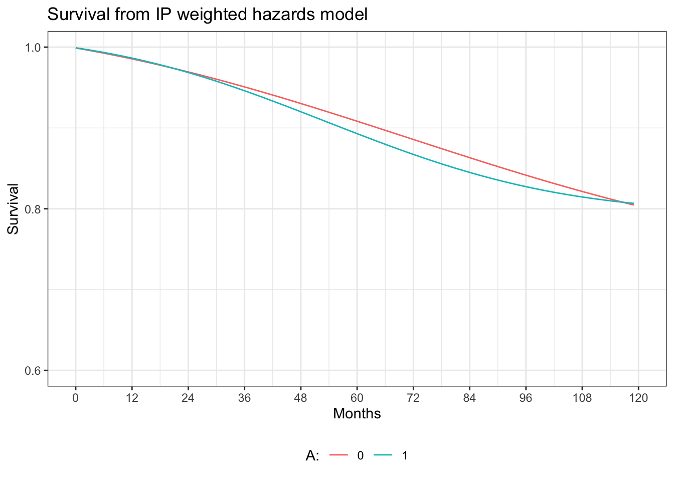
Program 17.4
- Estimating of survival curves via g-formula
- Data from NHEFS
# fit of hazards model with covariates
gf.model <- glm(event==0 ~ qsmk + I(qsmk*time) + I(qsmk*timesq)
                + time + timesq + sex + race + age + I(age*age)
                + as.factor(education) + smokeintensity
                + I(smokeintensity*smokeintensity) + smkintensity82_71
                + smokeyrs + I(smokeyrs*smokeyrs) + as.factor(exercise)
                + as.factor(active) + wt71 + I(wt71*wt71),
                data=nhefs.surv, family=binomial())
summary(gf.model)
#>
#> Call:
#> glm(formula = event == 0 ~ qsmk + I(qsmk * time) + I(qsmk * timesq) +
#>     time + timesq + sex + race + age + I(age * age) + as.factor(education) +
#>     smokeintensity + I(smokeintensity * smokeintensity) + smkintensity82_71 +
#>     smokeyrs + I(smokeyrs * smokeyrs) + as.factor(exercise) +
#>     as.factor(active) + wt71 + I(wt71 * wt71), family = binomial(),
#>     data = nhefs.surv)
#>
#> Coefficients:
#>                                      Estimate Std. Error z value Pr(>|z|)
#> (Intercept)                         9.272e+00  1.379e+00   6.724 1.76e-11 ***
#> qsmk                                5.959e-02  4.154e-01   0.143 0.885924
#> I(qsmk * time)                     -1.485e-02  1.506e-02  -0.987 0.323824
#> I(qsmk * timesq)                    1.702e-04  1.245e-04   1.367 0.171643
#> time                               -2.270e-02  8.437e-03  -2.690 0.007142 **
#> timesq                              1.174e-04  6.709e-05   1.751 0.080020 .
#> sex                                 4.368e-01  1.409e-01   3.101 0.001930 **
#> race                               -5.240e-02  1.734e-01  -0.302 0.762572
#> age                                -8.750e-02  5.907e-02  -1.481 0.138536
#> I(age * age)                        8.128e-05  5.470e-04   0.149 0.881865
#> as.factor(education)2               1.401e-01  1.566e-01   0.895 0.370980
#> as.factor(education)3               4.335e-01  1.526e-01   2.841 0.004502 **
#> as.factor(education)4               2.350e-01  2.790e-01   0.842 0.399750
#> as.factor(education)5               3.750e-01  2.386e-01   1.571 0.116115
#> smokeintensity                     -1.626e-03  1.430e-02  -0.114 0.909431
#> I(smokeintensity * smokeintensity) -7.182e-05  2.390e-04  -0.301 0.763741
#> smkintensity82_71                  -1.686e-03  6.501e-03  -0.259 0.795399
#> smokeyrs                           -1.677e-02  3.065e-02  -0.547 0.584153
#> I(smokeyrs * smokeyrs)             -5.280e-05  4.244e-04  -0.124 0.900997
#> as.factor(exercise)1                1.469e-01  1.792e-01   0.820 0.412300
#> as.factor(exercise)2               -1.504e-01  1.762e-01  -0.854 0.393177
#> as.factor(active)1                 -1.601e-01  1.300e-01  -1.232 0.218048
#> as.factor(active)2                 -2.294e-01  1.877e-01  -1.222 0.221766
#> wt71                                6.222e-02  1.902e-02   3.271 0.001073 **
#> I(wt71 * wt71)                     -4.046e-04  1.129e-04  -3.584 0.000338 ***
#> ---
#> Signif. codes:  0 '***' 0.001 '**' 0.01 '*' 0.05 '.' 0.1 ' ' 1
#>
#> (Dispersion parameter for binomial family taken to be 1)
#>
#>     Null deviance: 4655.3  on 176763  degrees of freedom
#> Residual deviance: 4185.7  on 176739  degrees of freedom
#> AIC: 4235.7
#>
#> Number of Fisher Scoring iterations: 10

# creation of dataset with all time points for
# each individual under each treatment level
gf.qsmk0 <- expandRows(nhefs, count=120, count.is.col=F)
gf.qsmk0$time <- rep(seq(0, 119), nrow(nhefs))
gf.qsmk0$timesq <- gf.qsmk0$time^2
gf.qsmk0$qsmk <- 0

gf.qsmk1 <- gf.qsmk0
gf.qsmk1$qsmk <- 1

gf.qsmk0$p.noevent0 <- predict(gf.model, gf.qsmk0, type="response")
gf.qsmk1$p.noevent1 <- predict(gf.model, gf.qsmk1, type="response")

#install.packages("dplyr")
library("dplyr")
#>
#> Attaching package: 'dplyr'
#> The following objects are masked from 'package:stats':
#>
#>     filter, lag
#> The following objects are masked from 'package:base':
#>
#>     intersect, setdiff, setequal, union
gf.qsmk0.surv <- gf.qsmk0 %>% group_by(seqn) %>% mutate(surv0 = cumprod(p.noevent0))
gf.qsmk1.surv <- gf.qsmk1 %>% group_by(seqn) %>% mutate(surv1 = cumprod(p.noevent1))

gf.surv0 <-
  aggregate(gf.qsmk0.surv,
            by = list(gf.qsmk0.surv$time),
            FUN = mean)[c("qsmk", "time", "surv0")]
gf.surv1 <-
  aggregate(gf.qsmk1.surv,
            by = list(gf.qsmk1.surv$time),
            FUN = mean)[c("qsmk", "time", "surv1")]

gf.graph <- merge(gf.surv0, gf.surv1, by=c("time"))
gf.graph$survdiff <- gf.graph$surv1-gf.graph$surv0

# plot
ggplot(gf.graph, aes(x=time, y=surv)) +
  geom_line(aes(y = surv0, colour = "0")) +
  geom_line(aes(y = surv1, colour = "1")) +
  xlab("Months") +
  scale_x_continuous(limits = c(0, 120), breaks=seq(0,120,12)) +
  scale_y_continuous(limits=c(0.6, 1), breaks=seq(0.6, 1, 0.2)) +
  ylab("Survival") +
  ggtitle("Survival from g-formula") +
  labs(colour="A:") +
  theme_bw() +
  theme(legend.position="bottom")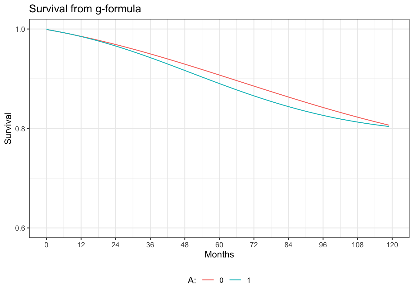
Program 17.5
- Estimating of median survival time ratio via a structural nested AFT model
- Data from NHEFS
# some preprocessing of the data
nhefs <- read_excel(here("data", "NHEFS.xls"))
nhefs$survtime <-
  ifelse(nhefs$death == 0, NA, (nhefs$yrdth - 83) * 12 + nhefs$modth)
  # * yrdth ranges from 83 to 92

# model to estimate E[A|L]
modelA <- glm(qsmk ~ sex + race + age + I(age*age)
              + as.factor(education) + smokeintensity
              + I(smokeintensity*smokeintensity) + smokeyrs
              + I(smokeyrs*smokeyrs) + as.factor(exercise)
              + as.factor(active) + wt71 + I(wt71*wt71),
              data=nhefs, family=binomial())

nhefs$p.qsmk <- predict(modelA, nhefs, type="response")
d <- nhefs[!is.na(nhefs$survtime),] # select only those with observed death time
n <- nrow(d)

# define the estimating function that needs to be minimized
sumeef <- function(psi){

  # creation of delta indicator
  if (psi>=0){
    delta <- ifelse(d$qsmk==0 |
                      (d$qsmk==1 & psi <= log(120/d$survtime)),
                    1, 0)
  } else if (psi < 0) {
    delta <- ifelse(d$qsmk==1 |
                      (d$qsmk==0 & psi > log(d$survtime/120)), 1, 0)
  }

  smat <- delta*(d$qsmk-d$p.qsmk)
  sval <- sum(smat, na.rm=T)
  save <- sval/n
  smat <- smat - rep(save, n)

  # covariance
  sigma <- t(smat) %*% smat
  if (sigma == 0){
    sigma <- 1e-16
  }
  estimeq <- sval*solve(sigma)*t(sval)
  return(estimeq)
}

res <- optimize(sumeef, interval = c(-0.2,0.2))
psi1 <- res$minimum
objfunc <- as.numeric(res$objective)


# Use simple bisection method to find estimates of lower and upper 95% confidence bounds
increm <- 0.1
for_conf <- function(x){
  return(sumeef(x) - 3.84)
}

if (objfunc < 3.84){
  # Find estimate of where sumeef(x) > 3.84

  # Lower bound of 95% CI
  psilow <- psi1
  testlow <- objfunc
  countlow <- 0
  while (testlow < 3.84 & countlow < 100){
    psilow <- psilow - increm
    testlow <- sumeef(psilow)
    countlow <- countlow + 1
  }

  # Upper bound of 95% CI
  psihigh <- psi1
  testhigh <- objfunc
  counthigh <- 0
  while (testhigh < 3.84 & counthigh < 100){
    psihigh <- psihigh + increm
    testhigh <- sumeef(psihigh)
    counthigh <- counthigh + 1
  }

  # Better estimate using bisection method
  if ((testhigh > 3.84) & (testlow > 3.84)){

    # Bisection method
    left <- psi1
    fleft <- objfunc - 3.84
    right <- psihigh
    fright <- testhigh - 3.84
    middle <- (left  + right) / 2
    fmiddle <- for_conf(middle)
    count <- 0
    diff <- right - left

    while (!(abs(fmiddle) < 0.0001 | diff < 0.0001 | count > 100)){
      test <- fmiddle * fleft
      if (test < 0){
        right <- middle
        fright <- fmiddle
      } else {
        left <- middle
        fleft <- fmiddle
      }
      middle <- (left + right) / 2
      fmiddle <- for_conf(middle)
      count <- count + 1
      diff <- right - left
    }

    psi_high <- middle
    objfunc_high <- fmiddle + 3.84

    # lower bound of 95% CI
    left <- psilow
    fleft <- testlow - 3.84
    right <- psi1
    fright <- objfunc - 3.84
    middle <- (left + right) / 2
    fmiddle <- for_conf(middle)
    count <- 0
    diff <- right - left

    while(!(abs(fmiddle) < 0.0001 | diff < 0.0001 | count > 100)){
      test <- fmiddle * fleft
      if (test < 0){
        right <- middle
        fright <- fmiddle
      } else {
        left <- middle
        fleft <- fmiddle
      }
      middle <- (left + right) / 2
      fmiddle <- for_conf(middle)
      diff <- right - left
      count <- count + 1
    }
    psi_low <- middle
    objfunc_low <- fmiddle + 3.84
    psi <- psi1
  }
}
c(psi, psi_low, psi_high)
#> [1] -0.05041591 -0.22312099  0.33312901