library(tidyverse)R, DOT, and TikZ code to plot directed acyclic graphs and single world intervention graphs for Mendelian randomization analyses
Introduction
This webpage shows some R code for generating figures, directed acyclic graphs (DAGs), and single world intervention graphs (SWIGs) for Mendelian randomization (MR) analyses.
First, we load in the tidyverse collection of packages to have access to the pipe and the ggplot2 package, amongst other features.
If you do not already one you will need a LaTeX installation. In R it is easiest to install TinyTeX as follows.
install.packages("tinytex")
tinytex::install_tinytex()
DiagrammeR package
The website for DiagrammeR is here: http://rich-iannone.github.io/DiagrammeR/ .
We will draw the DAGs using Graphviz which uses the DOT language to describe graphs.
Single genotype DAG
DiagrammeR::grViz("
  digraph mrdag {

  graph [rankdir=TB]

  node [shape=ellipse]
  U [label='Confounders']

  node [shape=box, height=0.3, width=0.3]
  G [label='Genotype']
  X [label='Phenotype']
  Y [label='Outcome']
  { rank = same; G X Y }

  G -> X [minlen=3]
  U -> X
  U -> Y
  X -> Y [minlen=3]
  }
  ", height = 200)
Version without borders around observed variables
DiagrammeR::grViz("
  digraph mrdag {

  graph [rankdir=TB]

  node [shape=ellipse]
  U [label='Confounders']

  node [shape=plaintext, height=0.3, width=0.3]
  G [label='Genotype']
  X [label='Phenotype']
  Y [label='Outcome']

  { rank = same; G X Y }

  G -> X [minlen=3]
  U -> X
  U -> Y
  X -> Y [minlen=3]
  }
  ", height = 200)
Multiple genotype DAG
DiagrammeR::grViz("
  digraph mrdag {

  graph [rankdir=TB, layout=neato]

  node [shape=ellipse]
  U [label='Confounders', pos='3,1!']

  node [shape=box, height=0.3, width=0.3]
  G1 [label='<I>G@_{1}</I>', pos='0,0.75!']
  G2 [label='<I>G@_{2}</I>', pos='0,0!']
  G3 [label='<I>G@_{3}</I>', pos='0,-0.75!']
  X [label='Phenotype', pos='2,0!']
  Y [label='Outcome', pos='4,0!']

  G1 -> X
  G2 -> X
  G3 -> X
  U -> X
  U -> Y
  X -> Y
  }
  ", height = 300)
This could be extended for more genotypes.
Version without borders around observed variables
DiagrammeR::grViz("
  digraph mrdag {

  graph [rankdir=TB, layout=neato]

  node [shape=ellipse]
  U [label='Confounders', pos='3,1!']

  node [shape=plaintext, height=0.3, width=0.3]
  G1 [label='<I>G@_{1}</I>', pos='0,0.75!']
  G2 [label='<I>G@_{2}</I>', pos='0,0!']
  G3 [label='<I>G@_{3}</I>', pos='0,-0.75!']
  X [label='Phenotype', pos='2,0!']
  Y [label='Outcome', pos='4,0!']

  G1 -> X
  G2 -> X
  G3 -> X
  U -> X
  U -> Y
  X -> Y
  }
  ", height = 300)
MVMR DAGs
We can plot the DAGs in Figure 4 of Sanderson et al. (2019) here.
Scenario 1: \(X_2\) confounder of \(X_1\) and \(Y\)
DiagrammeR::grViz("
  digraph mrdag {

  graph [rankdir=TB, layout=neato]

  node [shape=ellipse]
  U [label='Confounders', pos='3,1!']

  node [shape=plaintext, height=0.3, width=0.3]
  G1 [label='<I>G@_{1}</I>', pos='0,0!']
  X1 [label='<I>X@_{1}</I>', pos='2,0!']
  Y [label=<<I>Y</I>>, pos='4,0!']
  G2 [label='<I>G@_{2}</I>', pos='0,-1!']
  X2 [label='<I>X@_{2}</I>', pos='2,-1!']

  G1 -> X1
  G2 -> X2
  U -> X1
  U -> Y
  U -> X2
  X1 -> Y
  X2 -> Y
  X2 -> X1
  }
  ", height = 300)
Scenario 2: \(X_2\) collider of \(X_1\) and \(Y\)
DiagrammeR::grViz("
  digraph mrdag {

  graph [rankdir=TB, layout=neato]

  node [shape=ellipse]
  U [label='Confounders', pos='3,1!']

  node [shape=plaintext, height=0.3, width=0.3]
  G1 [label='<I>G@_{1}</I>', pos='0,0!']
  X1 [label='<I>X@_{1}</I>', pos='2,0!']
  Y [label=<<I>Y</I>>, pos='4,0!']
  G2 [label='<I>G@_{2}</I>', pos='0,-1!']
  X2 [label='<I>X@_{2}</I>', pos='2,-1!']

  G1 -> X1
  G2 -> X2
  U -> X1
  U -> Y
  U -> X2
  X1 -> Y
  Y -> X2
  X1 -> X2
  }
  ", height = 300)
Scenario 3: \(X_2\) on a pleiotropic pathway
DiagrammeR::grViz("
  digraph mrdag {

  graph [rankdir=TB, layout=neato]

  node [shape=ellipse]
  U [label='Confounders', pos='3,1!']

  node [shape=plaintext, height=0.3, width=0.3]
  G1 [label='<I>G@_{1}</I>', pos='0,0!']
  X1 [label='<I>X@_{1}</I>', pos='2,0!']
  Y [label=<<I>Y</I>>, pos='4,0!']
  G2 [label='<I>G@_{2}</I>', pos='0,-1!']
  X2 [label='<I>X@_{2}</I>', pos='2,-1!']

  G1 -> X1
  G2 -> X2
  U -> X1
  U -> Y
  U -> X2
  X1 -> Y
  X2 -> Y
  }
  ", height = 300)
Scenario 4: \(X_2\) mediator of the effect of \(X_1\) on \(Y\)
DiagrammeR::grViz("
  digraph mrdag {

  graph [rankdir=TB, layout=neato]

  node [shape=ellipse]
  U [label='Confounders', pos='3,1!']

  node [shape=plaintext, height=0.3, width=0.3]
  G1 [label='<I>G@_{1}</I>', pos='0,0!']
  X1 [label='<I>X@_{1}</I>', pos='2,0!']
  Y [label=<<I>Y</I>>, pos='4,0!']
  G2 [label='<I>G@_{2}</I>', pos='0,-1!']
  X2 [label='<I>X@_{2}</I>', pos='2,-1!']

  edge [arrowhead='vee']
  G1 -> X1
  G2 -> X2
  U -> X1
  U -> Y
  U -> X2
  X1 -> Y
  X2 -> Y
  X1 -> X2
  }
  ", height = 300)
Bidirectional MR figure of combined DAGs
For a bidirectional MR analysis there are 2 separate DAGs which are as follows.
DiagrammeR::grViz("
  digraph mrdag {

  graph [rankdir=TB, layout=neato]

  node [shape=ellipse]
  U [label='Confounders', pos='3,1!']

  node [shape=plaintext, height=0.3, width=0.3]
  GX [label='Genotypes \n for phenotype', pos='0,0!']
  X [label='Phenotype', pos='2,0!']
  Y [label='Outcome', pos='4,0!']

  GX -> X [penwidth=2]
  U -> X [penwidth=2]
  U -> Y [penwidth=2]
  X -> Y [penwidth=2]
  }
", height = 200)DiagrammeR::grViz("
digraph mrdag {
graph [rankdir=TB, layout=neato]
node [shape=ellipse]
U [label='Confounders', pos='3,1!']
node [shape=plaintext, height=0.3, width=0.3]
X [label='Phenotype', pos='2,0!']
Y [label='Outcome', pos='4,0!']
GY [label='Genotypes \n for outcome', pos='6,0!']
U -> X [penwidth=2]
U -> Y [penwidth=2]
Y -> X [penwidth=2]
GY -> Y [penwidth=2]
}
", height = 200)We can combine these into a single figure as follows.
DiagrammeR::grViz("
  digraph mrdag {

  graph [rankdir=TB, layout=neato]

  node [shape=ellipse]
  U [label='Confounders', pos='3,1!']

  node [shape=plaintext, height=0.3, width=0.3]
  GX [label='Genotypes \n for phenotype', pos='0,0!']
  X [label='Phenotype', pos='2,0!']
  Y [label='Outcome', pos='4,0!']
  GY [label='Genotypes \n for outcome', pos='6,0!']

  { rank = same; GX X Y GY }

  GX -> X [penwidth=2]
  U -> X [penwidth=2]
  U -> Y [penwidth=2]
  X -> Y [penwidth=2]
  Y -> X [color=blue, penwidth=2]
  GY -> Y [color=blue, penwidth=2]
  }
  ", height = 200)
Arguably we could add additional blue arrows from the Confounders node.
If you prefer a greyscale figure replace blue with grey/DimGrey/grey30 (or change the number as required. See here for more colors.
Pleiotropy DAGs
There are many types of pleiotropy. Let’s plot some of the pleiotropy DAGs from Sanderson et al. (2022).
Horizontal pleiotropy (causes bias)
DiagrammeR::grViz("
  digraph mrdag {

  graph [rankdir=TB]

  node [shape=ellipse]
  U [label='Confounders']

  node [shape=plaintext, height=0.3, width=0.3]
  G [label='Genotype']
  X [label='Phenotype']
  Y [label='Outcome']
  C [label='Other phenotype']

  { rank = same; G X Y }

  G -> X [minlen=3]
  G -> C
  U -> X
  U -> Y
  X -> Y [minlen=3]
  C -> Y
  }
  ", height = 300)
Horizontal pleiotropy (no bias)
DiagrammeR::grViz("
  digraph mrdag {

  graph [rankdir=TB, layout=neato]

  node [shape=ellipse]
  U [label='Confounders', pos='3,1!']

  node [shape=plaintext, height=0.3, width=0.3]
  G [label='Genotype', pos='0,0!']
  X [label='Phenotype', pos='2,0!']
  Y [label='Outcome', pos='4,0!']
  C [label='Other phenotype', pos='2,-1!']

  G -> X
  G -> C
  U -> X
  U -> Y
  X -> Y
  }
  ", height = 300)
Confounding via linkage disequilibrium
DiagrammeR::grViz("
  digraph mrdag {

  graph [rankdir=TB, layout=neato]

  node [shape=ellipse]
  U [label='Confounders', pos='3,1!']

  node [shape=plaintext, height=0.3, width=0.3]
  G1 [label='Genotype 1', pos='0,0!']
  G2 [label='Genotype 2', pos='0,-1!']
  X [label='Phenotype', pos='2,0!']
  Y [label='Outcome', pos='4,0!']
  C [label='Other phenotype', pos='2,-1!']

  G1 -> X
  G1 -> G2 [dir='both']
  G2 -> C
  U -> X
  U -> Y
  X -> Y
  C -> Y
  }
  ", height = 300)
Vertical pleiotropy
DiagrammeR::grViz("
  digraph mrdag {

  graph [rankdir=TB]

  node [shape=ellipse]
  U [label='Confounders']

  node [shape=plaintext, height=0.3, width=0.3]
  G [label='Genotype']
  X [label='Phenotype 1']
  Y [label='Outcome']
  C [label='Phenotype 2']

  { rank = same; G X C Y }

  G -> X [minlen=2]
  X -> C [minlen=2]
  U -> X
  U -> Y
  C -> Y [minlen=2]
  }
  ", height = 200)
Misspecification of the primary phenotype
DiagrammeR::grViz("
  digraph mrdag {

  graph [rankdir=TB, layout=neato]

  node [shape=ellipse]
  U [label='Confounders', pos='3,1!']

  node [shape=plaintext, height=0.3, width=0.3]
  G [label='Genotype', pos='0,0!']
  X [label='Phenotype 1', pos='2,0!']
  Y [label='Outcome', pos='4,0!']
  C [label='Phenotype 2', pos='2,-1!']

  G -> C
  C -> X
  U -> X
  U -> Y
  X -> Y
  C -> Y
  }
", height = 300)Single genotype path diagram
Explicitly including the confounder
DiagrammeR::grViz("
digraph mrdag {
graph [rankdir=TB, layout=neato]
node [shape=ellipse, height=0.3, width=0.3]
U [label=<<I>U</I>>, pos='3,1!']
node [shape=box, height=0.3, width=0.3]
G [label=<<I>G</I>>, pos='0,0!']
X [label=<<I>X</I>>, pos='2,0!']
Y [label=<<I>Y</I>>, pos='4,0!']
node [shape=circle, height=0.35, fixedsize=true]
Ex [label='<I>ε@_{X}</I>', pos='2,1!']
Ey [label='<I>ε@_{Y}</I>', pos='4,1!']
G -> X [label='<I>β@_{GX}</I>']
Ex -> X [label=1]
Ey -> Y [label=1]
U -> X [label='<I>β@_{UX}</I>']
U -> Y [label='<I>β@_{UY}</I>']
X -> Y [label='<I>β@_{XY}</I>']
U -> U [dir='both', headport='n', tailport='n']
G -> G [dir='both', headport='w', tailport='w']
}
", height = 250)Including variance terms
Note in the diagram below \(\sigma_{X}^2\) and \(\sigma_{Y}^2\) represent the variance of the respective error/residual terms (\(\varepsilon_X\), \(\varepsilon_Y\)) and not the variance of \(X\) and \(Y\).
DiagrammeR::grViz("
digraph mrdag {
graph [rankdir=TB, layout=neato]
node [shape=ellipse, height=0.3, width=0.3]
U [label=<<I>U</I>>, pos='3,1!']
node [shape=box, height=0.3, width=0.3]
G [label=<<I>G</I>>, pos='0,0!']
X [label=<<I>X</I>>, pos='2,0!']
Y [label=<<I>Y</I>>, pos='4,0!']
node [shape=circle, height=0.35, fixedsize=true]
Ex [label='<I>ε@_{X}</I>', pos='2,1!']
Ey [label='<I>ε@_{Y}</I>', pos='4,1!']
G -> X [label='<I>β@_{GX}</I>']
Ex -> X [label=1]
Ey -> Y [label=1]
U -> X [label='<I>β@_{UX}</I>']
U -> Y [label='<I>β@_{UY}</I>']
X -> Y [label='<I>β@_{XY}</I>']
U -> U [dir='both', headport='n', tailport='n', label=<var(<I>U</I>)>]
G -> G [dir='both', headport='w', tailport='w', label=<var(<I>G</I>)>]
Ex -> Ex [dir='both', headport='n', tailport='n', label=<<I>σ@_{X}@^{2}</I>>]
Ey -> Ey [dir='both', headport='n', tailport='n', label=<<I>σ@_{Y}@^{2}</I>>]
}
", height = 250)dagitty package
The website for DAGitty is http://www.dagitty.net/
library(dagitty)Using DOT syntax
The DAG for a single genotype.
mrdag <- dagitty('dag {
  G -> X -> Y
  X <- U -> Y
  G [pos="0,0"]
  X [e, pos="1,0"]
  U [pos="1.5,-0.4"]
  Y [o, pos="2,0"]
}')

plot(mrdag)
Using ggdag
library(ggdag)
mrdag <- dagitty('dag {
  G -> X -> Y
  X <- U -> Y
  G [pos="0,0"]
  X [e, pos="1,0"]
  U [pos="1.5,0.4"]
  Y [o, pos="2,0"]
}')

ggmrdag <- tidy_dagitty(mrdag)
ggdag(ggmrdag) + theme_dag()
This can be labelled as follows.
mrdag <- mrdag |>
  dag_label(
    labels = c(
      "X" = "Exposure",
      "Y" = "Outcome",
      "G" = "Genotype",
      "U" = "Confounders"))
ggdag(mrdag,  use_labels = "label") + theme_dag()
Dagitty can identify the instrumental variable on the DAG.
mrdag |> ggdag_instrumental() + theme_dag()
It correctly identifies the genotype, \(G\), as the instrumental variable.
Using the dagitty web interface
We can draw the MR DAG in the dagitty web interface https://www.dagitty.net/dags.html.
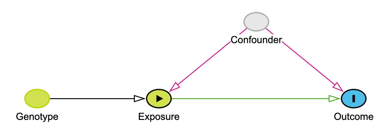
The code is very similar to that above, except that the position values are different.
dag {
  bb="0,0,1,1"
  "Instrumental variable" [pos="0.150,0.200"]
  Confounder [latent,pos="0.600,0.100"]
  Exposure [exposure,pos="0.400,0.200"]
  Outcome [outcome,pos="0.800,0.200"]
  "Instrumental variable" -> Exposure
  Confounder -> Exposure
  Confounder -> Outcome
  Exposure -> Outcome
}
And dagitty also gives the tikz code.
% This code uses the tikz package
\begin{tikzpicture}
\node (v0) at (0.150,-0.200) {Instrumental variable};
\node (v1) at (0.600,-0.100) {Confounder};
\node (v2) at (0.400,-0.200) {Exposure};
\node (v3) at (0.800,-0.200) {Outcome};
\draw [->] (v0) edge (v2);
\draw [->] (v1) edge (v2);
\draw [->] (v1) edge (v3);
\draw [->] (v2) edge (v3);
\end{tikzpicture}
This DAG is saved and available at https://dagitty.net/dags.html?id=q2va7XkL.
Using R model type syntax in ggdag
coords <- list(x = c(G = 0, X = 1, Y = 2, U = 1.5),
               y = c(G = 0, X = 0, Y = 0, U = 1))
mrdag <- dagify(
  X ~ G + U,
  Y ~ X + U,
  labels = c(
    "G" = "Genotype",
    "X" = "Exposure",
    "Y" = "Outcome",
    "U" = "Confounders"
  ),
  exposure = "X",
  outcome = "Y",
  coords = coords
)
ggdag(mrdag, use_labels = "label") + theme_dag()
Plotting directly with ggplot2 functions.
mrdag |>
  ggplot(aes(
    x = x,
    y = y,
    xend = xend,
    yend = yend
  )) +
  geom_dag_point() +
  geom_dag_edges() +
  geom_dag_text() +
  theme_dag()
Showing the paths.
set.seed(123)
dagify(Y ~ X + U,
       X ~ U + G,
       exposure = "X",
       outcome = "Y") |>
ggdag_paths() + theme_dag()
Adjustment set for the effect of \(X\) on \(Y\).
dagify(Y ~ X + U,
       X ~ U + G,
       exposure = "X",
       outcome = "Y",
       coords = coords) |>
  ggdag_adjustment_set() + theme_dag()
This shows that the path from \(G\) to \(X\) is unconfounded. And that when \(U\) is adjusted for the path from \(X\) to \(Y\) is unconfounded.
Multiple genotype DAG
coords2 <- list(x = c(G1 = 0, G2 = 0, G3 = 0, X = 1, Y = 2, U = 1.5),
                y = c(G1 = 0.5, G2 = 0, G3 = -0.5, X = 0, Y = 0, U = 1))
mrdag <- dagify(
  X ~ G1,
  X ~ G2,
  X ~ G3,
  Y ~ X,
  X ~ U,
  Y ~ U,
  exposure = "X",
  outcome = "Y",
  coords = coords2
)
ggdag(mrdag) + theme_dag()
This could be extended for more genotypes.
Eleanor Murray’s TikZ diagrams using the tikz code chunk engine
I believe that tikz diagrams can be included in Rmarkdown documents using the tikz code chunk engine for output types pdf_document and html_document.
Tikz is a package for LaTeX and so pdf is its natural output. So far I have not been able to include these figures in either html_notebook or word_document output formats. I suspect that the images need conversion to png files for these to work under rmarkdown.
We will use some of the LaTeX code for drawing DAGs using tikz provided by Eleanor Murray here.
In its LaTeX preamble, this code loads in several TikZ libraries. As such for our tikz code chunks to compile in our Rmd file we need to define a new template file, e.g.tikz-template.tex, and call our tikz code chunks as follows.
```{tikz}
%| out-width: "65%"
%| engine-opts:
%|   template: "tikz-template.tex"
%|   dvisvgm.opts: "--font-format=woff"
\begin{tikzpicture}
% Your tikz code goes here ...
\end{tikzpicture}
```
The tikz-template.tex file includes the TikZ preamble code from Eleanor Murray’s LaTeX code plus the required template code. The contents of the template file is as follows.
\documentclass{article}
\usepackage[active, tightpage]{preview}
\usepackage{amsmath}
\usepackage{tikz}
\usetikzlibrary{positioning, calc, shapes.geometric, shapes.multipart,
    shapes, arrows.meta, arrows, decorations.markings, external, trees}

% Create custom arrow style:
\tikzstyle{Arrow} = [
  thick,
  decoration={markings,
              mark=at position 1 with {\arrow[thick]{latex}}},
  shorten >= 3pt,
  preaction = {decorate}
]

\tikzstyle{BlueArrow} = [
  thick,
  decoration={markings,
              mark=at position 1 with {\arrow[thick, blue]{latex}}},
  shorten >= 3pt,
  preaction = {decorate},
  color = blue
]

\begin{document}
\begin{preview}
%% TIKZ_CODE %%
\end{preview}
\end{document}
We can now plot our DAGs.
Single genotype DAGs using TikZ
Specifying node coordinates
\begin{tikzpicture}
\node (1) at (0,0) {$G$};
\node (2) at (1.5,0) {$X$};
\node (3) at (3,0) {$Y$};
\node (4) at (2.25,1) {$U$};
\draw[Arrow] (1) -- (2);
\draw[Arrow] (2) -- (3);
\draw[Arrow] (4) -- (2);
\draw[Arrow] (4) -- (3);
\end{tikzpicture}
Single genotype DAG using tikz-cd
The tikz-cd package provides helpful syntax for making commutative diagrams which we can use to produce DAGs.
First install the package.
tinytex::tlmgr_install("tikz-cd")Then we can plot the single instrument DAG using the following code.
\usetikzlibrary{cd}
\tikzcdset{arrow style=tikz, diagrams={>=stealth}}
\begin{tikzcd}[column sep=tiny]
& & & & U \arrow[dl, thick] \arrow[dr, thick] & \\
G \arrow[thick]{rrr} & & & X \arrow[thick]{rr} & & Y
\end{tikzcd}
Single genotype DAG using simpler TikZ code
\usetikzlibrary{positioning}
\tikzset{
    > = stealth,
    every path/.append style = {
        arrows = ->,
        thick
    }
}
\tikz{
    \node (g) {$G$};
    \node (x) [right = of g] {$X$};
    \node (y) [right = of x] {$Y$};
    \node (u) [above right = 0.5cm and 0.25cm of x] {$U$};
    \path (g) edge (x);
    \path (x) edge (y);
    \path (u) edge (x);
    \path (u) edge (y);
}
Multiple genotype DAGs using TikZ
Specifying node coordinates
\begin{tikzpicture}
\node (1) at (0,0) {$G_2$};
\node (2) at (1.5,0) {$X$};
\node (3) at (3,0) {$Y$};
\node (4) at (2.25,1) {$U$};
\node (5) at (0,0.5) {$G_1$};
\node (6) at (0,-0.5) {$G_3$};
\draw[Arrow] (1) -- (2);
\draw[Arrow] (2) -- (3);
\draw[Arrow] (4) -- (2);
\draw[Arrow] (4) -- (3);
\draw[Arrow] (5) -- (2);
\draw[Arrow] (6) -- (2);
\end{tikzpicture}
Again this could be extended for more genotypes.
Multiple genotype DAG using circularly spaced genotypes
\begin{tikzpicture}
\node (1) at (0,0) {$G_2$};
\node (2) at (1.5,0) {$X$};
\node (3) at (3,0) {$Y$};
\node (4) at (2.25,1) {$U$};
\node (5) at ([shift=({160:1.5})]2) {$G_1$};
\node (6) at ([shift=({200:1.5})]2) {$G_3$};
\draw[Arrow] (1) -- (2);
\draw[Arrow] (2) -- (3);
\draw[Arrow] (4) -- (2);
\draw[Arrow] (4) -- (3);
\draw[Arrow] (5) -- (2);
\draw[Arrow] (6) -- (2);
\end{tikzpicture}
Pleiotropy DAGs using TikZ
Horizontal pleiotropy (causes bias)
\usetikzlibrary{positioning}
\tikzset{
    > = stealth,
    every path/.append style = {
        arrows = ->,
        thick
    }
}
\tikz{
    \node (g) {$G$};
    \node (x1) [right = of g] {$X_1$};
    \node (y) [right = of x1] {$Y$};
    \node (u) [above right = 0.5cm and 0.25cm of x1] {$U$};
    \node (x2) [below = 0.5cm of x1] {$X_2$};
    \path (g) edge (x1);
    \path (x1) edge (y);
    \path (u) edge (x1);
    \path (u) edge (y);
    \path (g) edge (x2);
    \path (x2) edge (y);
}
Horizontal pleiotropy (no bias)
\usetikzlibrary{positioning}
\tikzset{
    > = stealth,
    every path/.append style = {
        arrows = ->,
        thick
    }
}
\tikz{
    \node (g) {$G$};
    \node (x1) [right = of g] {$X_1$};
    \node (y) [right = of x1] {$Y$};
    \node (u) [above right = 0.5cm and 0.25cm of x1] {$U$};
    \node (x2) [below = 0.5cm of x1] {$X_2$};
    \path (g) edge (x1);
    \path (x1) edge (y);
    \path (u) edge (x1);
    \path (u) edge (y);
    \path (g) edge (x2);
}
Confounding via linkage disequilibrium
\usetikzlibrary{positioning}
\tikzset{
    > = stealth,
    every path/.append style = {
        arrows = ->,
        thick
    }
}
\tikz{
    \node (g1) {$G_1$};
    \node (x1) [right = of g1] {$X_1$};
    \node (y) [right = of x1] {$Y$};
    \node (u) [above right = 0.5cm and 0.25cm of x1] {$U$};
    \node (x2) [below = 0.5cm of x1] {$X_2$};
    \node (g2) [below = 0.5cm of g1] {$G_2$};
    \path (g1) edge (x1);
    \path (x1) edge (y);
    \path (u) edge (x1);
    \path (u) edge (y);
    \draw[<->] (g1) -- (g2);
    \path (g2) edge (x2);
    \path (x2) edge (y);
}
Vertical pleiotropy
\usetikzlibrary{positioning}
\tikzset{
    > = stealth,
    every path/.append style = {
        arrows = ->,
        thick
    }
}
\tikz{
    \node (g) {$G$};
    \node (x1) [right = of g] {$X_1$};
    \node (x2) [right = of x1] {$X_2$};
    \node (y) [right = of x2] {$Y$};
    \node (u) [above = 0.5cm of x2] {$U$};
    \path (g) edge (x1);
    \path (x1) edge (x2);
    \path (u) edge (x1);
    \path (u) edge (y);
    \path (x2) edge (y);
}
Misspecification of the primary phenotype
\usetikzlibrary{positioning}
\tikzset{
    > = stealth,
    every path/.append style = {
        arrows = ->,
        thick
    }
}
\tikz{
    \node (g) {$G$};
    \node (x1) [right = of g] {$X_1$};
    \node (y) [right = of x1] {$Y$};
    \node (u) [above right = 0.5cm and 0.25cm of x1] {$U$};
    \node (x2) [below = 0.5cm of x1] {$X_2$};
    \path (x1) edge (y);
    \path (u) edge (x1);
    \path (u) edge (y);
    \path (g) edge (x2);
    \path (x2) edge (x1);
    \path (x2) edge (y);
}
Correlated pleiotropy
\usetikzlibrary{positioning}
\tikzset{
    > = stealth,
    every path/.append style = {
        arrows = ->,
        thick
    }
}
\tikz{
    \node (g) {$G$};
    \node (x1) [right = of g] {$X_1$};
    \node (y) [right = of x1] {$Y$};
    \node (u) [above right = 0.5cm and 0.25cm of x1] {$U$};
    \node (x2) [below = 0.5cm of x1] {$X_2$};
    \path (x1) edge (y);
    \path (u) edge (x1);
    \path (u) edge (y);
    \path (g) edge (x2);
    \path (x2) edge (x1);
    \path (x2) edge (y);
    \path (g) edge (x1);
    \path (g) edge (x2);
}
Bidirectional MR figure of combined DAGs using TikZ
For a bidirectional MR analysis there are 2 separate DAGs, which are as follows.
\begin{tikzpicture}
\node (1) at (0,0) {$G_X$};
\node (2) at (1.5,0) {$X$};
\node (3) at (3,0) {$Y$};
\node (4) at (2.25,1) {$U$};
\draw[Arrow] (1) -- (2);
\draw[Arrow] (2) -- (3);
\draw[Arrow] (4) -- (2);
\draw[Arrow] (4) -- (3);
\end{tikzpicture}
\begin{tikzpicture}
\node (2) at (1.5,0) {$X$};
\node (3) at (3,0) {$Y$};
\node (4) at (2.25,1) {$U$};
\node (5) at (4.5,0) {$G_Y$};
\draw[Arrow] (3) -- (2);
\draw[Arrow] (4) -- (2);
\draw[Arrow] (4) -- (3);
\draw[Arrow] (5) -- (3);
\end{tikzpicture}
We can combine these into a single figure as follows.
\begin{tikzpicture}
\node (1) at (0,0) {$G_X$};
\node (2) at (1.5,0) {$X$};
\node (3) at (3,0) {$Y$};
\node (4) at (2.25,1) {$U$};
\node (5) at (4.5,0) {$G_Y$};
% Create dummy X and Y nodes with no content
\node (6) at (1.5,-0.05) {\phantom{$X$}};
\node (7) at (3,-0.05) {\phantom{$Y$}};
\node (8) at (1.5,0.05) {\phantom{$X$}};
\node (9) at (3,0.05) {\phantom{$Y$}};
\draw[Arrow] (1) -- (2);
\draw[Arrow] (8) -- (9);
\draw[BlueArrow] (7) -- (6);
\draw[Arrow] (4) -- (2);
\draw[Arrow] (4) -- (3);
\draw[BlueArrow] (5) -- (3);
\end{tikzpicture}
MVMR DAGs using TikZ
We can plot the DAGs in Figure 4 of Sanderson et al. (2019) here.
Scenario 1: \(X_2\) confounder of \(X_1\) and \(Y\)
\begin{tikzpicture}
\node (1) at (0,0) {$G_2$};
\node (2) at (1.5,0) {$X_2$};
\node (3) at (4.5,1) {$Y$};
\node (4) at (3,2) {$U$};
\node (5) at (0,1) {$G_1$};
\node (6) at (1.5,1) {$X_1$};
\draw[Arrow] (1) -- (2);
\draw[Arrow] (2) -- (3);
\draw[Arrow] (4) -- (2);
\draw[Arrow] (4) -- (3);
\draw[Arrow] (5) -- (6);
\draw[Arrow] (6) -- (3);
\draw[Arrow] (4) -- (6);
\draw[Arrow] (2) -- (6);
\end{tikzpicture}
Scenario 2: \(X_2\) collider of \(X_1\) and \(Y\)
\begin{tikzpicture}
\node (1) at (0,0) {$G_2$};
\node (2) at (1.5,0) {$X_2$};
\node (3) at (4.5,1) {$Y$};
\node (4) at (3,2) {$U$};
\node (5) at (0,1) {$G_1$};
\node (6) at (1.5,1) {$X_1$};
\draw[Arrow] (1) -- (2);
\draw[Arrow] (3) -- (2);
\draw[Arrow] (4) -- (2);
\draw[Arrow] (4) -- (3);
\draw[Arrow] (5) -- (6);
\draw[Arrow] (6) -- (3);
\draw[Arrow] (4) -- (6);
\draw[Arrow] (6) -- (2);
\end{tikzpicture}
Scenario 3: \(X_2\) on a pleiotropic pathway
\begin{tikzpicture}
\node (1) at (0,0) {$G_2$};
\node (2) at (1.5,0) {$X_2$};
\node (3) at (4.5,1) {$Y$};
\node (4) at (3,2) {$U$};
\node (5) at (0,1) {$G_1$};
\node (6) at (1.5,1) {$X_1$};
\draw[Arrow] (1) -- (2);
\draw[Arrow] (2) -- (3);
\draw[Arrow] (4) -- (2);
\draw[Arrow] (4) -- (3);
\draw[Arrow] (5) -- (6);
\draw[Arrow] (6) -- (3);
\draw[Arrow] (4) -- (6);
\end{tikzpicture}
Scenario 4: \(X_2\) mediator of the effect of \(X_1\) on \(Y\)
\begin{tikzpicture}
\node (1) at (0,0) {$G_2$};
\node (2) at (1.5,0) {$X_2$};
\node (3) at (4.5,1) {$Y$};
\node (4) at (3,2) {$U$};
\node (5) at (0,1) {$G_1$};
\node (6) at (1.5,1) {$X_1$};
\draw[Arrow] (1) -- (2);
\draw[Arrow] (2) -- (3);
\draw[Arrow] (4) -- (2);
\draw[Arrow] (4) -- (3);
\draw[Arrow] (5) -- (6);
\draw[Arrow] (6) -- (3);
\draw[Arrow] (4) -- (6);
\draw[Arrow] (6) -- (2);
\end{tikzpicture}
quickdag package
We can produce some nice plots with the quickdag package, which appears to be based on Eleanor Murray’s TikZ code, from here
Single genotype DAG
# if (!require("quickdag")) remotes::install_github("jrgant/quickdag")
library(quickdag)
library(DiagrammeR)
edges <- c("G -> X",
           "X -> Y",
           "U -> {X Y}")
# DAG
dag  <- qd_dag(edges, verbose = FALSE)
dag |> render_graph()
Single genotype SWIG
We can also draw the single world intervention graph (SWIG) for the IV model as follows.
swig <- dag |>
  qd_swig(fixed_nodes = c("G", "X"))
swig |> render_graph()
Thomas Richardson’s TikZ code for SWIGs
Thomas Richardson provides a TikZ/PGF shape library for SWIGs called tikz-swigs, which is available on CTAN here.
Install the package into your TinyTeX installation with
tinytex::tlmgr_install("tikz-swigs")Its user manual is available here
To use the tikz chunk engine we again write a LaTeX template based on the preamble in the article by Richardson. The LaTeX template is as follows.
\documentclass{article}
\usepackage[active, tightpage]{preview}
\usepackage{amsmath}
\usepackage{pgf, tikz}
\usetikzlibrary{arrows, shapes.arrows, shapes.geometric, shapes.multipart,
decorations.pathmorphing, positioning, swigs}

\begin{document}
\begin{preview}
%% TIKZ_CODE %%
\end{preview}
\end{document}
The simple SWIG for confounding
\begin{tikzpicture}
\tikzset{line width=1.5pt, outer sep=0pt,
  ell/.style={draw, fill=white, inner sep=2pt,
  line width=1.5pt},
  swig vsplit={gap=5pt, inner line width right=0.5pt},
  swig hsplit={gap=5pt, inner line width lower=0.5pt}};

\node[name=X,
  shape=swig vsplit,
  swig vsplit = {line color right=red,
                 line width right=2.5pt}]{
\nodepart{left}{$X$}
\nodepart{right}{\textcolor{red}{$x$}}};

\node[name=U, ell, shape=ellipse, above right=7.5mm and 5mm of X, fill=gray]{$U$};

\node[name=Y, ell, shape=ellipse, right=10mm of X]{$Y^{\textcolor{red}{x}}$};

\draw[->, line width=1.5pt,>=stealth, color=blue]
  (U) edge[out=220, in=120] (X)
  (U) edge (Y)
  (X) to (Y);
\end{tikzpicture}
SWIGs for single exposure models
We will recreate the SWIG template in Figure 2 (b) of Swanson et al. here.
\begin{tikzpicture}
\tikzset{line width=1.5pt, outer sep=0pt,
  ell/.style={draw, fill=white, inner sep=2pt,
  line width=1.5pt},
  swig vsplit={gap=5pt, inner line width right=0.5pt},
  swig hsplit={gap=5pt, inner line width lower=0.5pt}};

\node[name=G, shape=swig vsplit]{
\nodepart{left}{$G$}
\nodepart{right}{$g$}};

\node[name=X, right=10mm of G,
  shape=swig hsplit]{
\nodepart{upper}{$X^g$}
\nodepart{lower}{$x$}};

\node[name=U, ell, shape=ellipse, above right=7.5mm and 5mm of X, fill=gray]{$U$};

\node[name=Y, ell, shape=ellipse, right=10mm of X]{$Y^x$};

\draw[->, line width=1.5pt,>=stealth]
  (G) edge[out=360, in=170] (X)
  (U) edge (X)
  (U) edge (Y)
  (X) to[out=330, in=180] (Y);
\end{tikzpicture}
Let’s add colour in the same way as in the original figure.
\begin{tikzpicture}
\tikzset{line width=1.5pt, outer sep=0pt,
  ell/.style={draw, fill=white, inner sep=2pt,
  line width=1.5pt},
  swig vsplit={gap=5pt, inner line width right=0.5pt},
  swig hsplit={gap=5pt, inner line width lower=0.5pt}};

\node[name=G, shape=swig vsplit,
  swig vsplit={line color right=red,
               line width right=2.5pt}]{
\nodepart{left}{$G$}
\nodepart{right}{\textcolor{red}{$g$}}};

\node[name=X, right=10mm of G,
  shape=swig hsplit,
  swig hsplit = {line color lower=red,
                 line width lower=2.5pt}]{
\nodepart{upper}{$X^{\textcolor{red}{g}}$}
\nodepart{lower}{\textcolor{red}{$x$}}};

\node[name=U, ell, shape=ellipse, above right=7.5mm and 5mm of X, fill=gray]{$U$};

\node[name=Y, ell, shape=ellipse, right=10mm of X]{$Y^{\textcolor{red}{x}}$};

\draw[->, line width=1.5pt,>=stealth, color=blue]
  (G) edge[out=360, in=170] (X)
  (U) edge (X)
  (U) edge (Y)
  (X) to[out=330, in=180] (Y);
\end{tikzpicture}
SWIGs for MVMR models
Let’s attempt the SWIG for the multivariable Mendelian randomization (MVMR) model.
SWIG for MVMR model with 2 independent exposures
Since \(G_1\) an instrument for both \(X_1\) and \(X_2\), \(X_2\) represents a pleiotropic effect in this case.
\begin{tikzpicture}
\tikzset{line width=1.5pt, outer sep=0pt,
  ell/.style={draw, fill=white, inner sep=2pt,
  line width=1.5pt},
  swig vsplit={gap=5pt},
  swig hsplit={gap=5pt, inner line width lower=0.5pt}};

\node[name=G1,
  shape=swig vsplit,
  swig vsplit={line color right=red}]{
\nodepart{left}{$G_1$}
\nodepart{right}{\textcolor{red}{$g_1$}}};

\node[name=X1,
  right=10mm of G1,
  shape=swig hsplit,
  swig hsplit = {line color lower=red,
                 line width lower=2.5pt}]{
\nodepart{upper}{$X_1^{\phantom{1}\textcolor{red}{g_1,\,g_2}}$}
\nodepart{lower}{\textcolor{red}{$x_1$}}};

\node[name=X2,
  below = 1mm of X1,
  shape=swig hsplit,
  swig hsplit = {line color lower=red,
                 line width lower=2.5pt}]{
\nodepart{upper}{$X_2^{\phantom{2}\textcolor{red}{g_1,\,g_2}}$}
\nodepart{lower}{\textcolor{red}{$x_2$}}};

\node[name=G2,
  left = 10mm of X2,
  shape=swig vsplit,
  swig vsplit={line color right=red}]{
\nodepart{left}{$G_2$}
\nodepart{right}{\textcolor{red}{$g_2$}}};

\node[name=U,
  ell,
  shape=ellipse,
  above right=7.5mm and 5mm of X1,
  fill=gray]{$U$};

\node[name=Y,
  ell,
  shape=ellipse,
  below right=2mm and 20mm of X1]{$Y^{\textcolor{red}{x_1, x_2}}$};

\draw[->, line width=1.5pt,>=stealth, color=blue]
  (G1) edge[out=360, in=150] (X1)
  (G1) edge[out=360, in=150] (X2)
  (G2) edge[out=360, in=170] (X2)
  (G2) edge[out=360, in=170] (X1)
  (U) edge (X1)
  (U) edge[out=270, in=45] (X2)
  (U) edge (Y)
  (X1) edge[out=330, in=170] (Y)
  (X2) to[out=330, in=190] (Y);
\end{tikzpicture}
SWIG for MVMR model with \(X_2\) confounder of \(X_1\)–\(Y\)
\begin{tikzpicture}
\tikzset{line width=1.5pt, outer sep=0pt,
  ell/.style={draw, fill=white, inner sep=2pt,
  line width=1.5pt},
  swig vsplit={gap=5pt},
  swig hsplit={gap=5pt, inner line width lower=0.5pt}};

\node[name=G1,
  shape=swig vsplit,
  swig vsplit={line color right=red}]{
\nodepart{left}{$G_1$}
\nodepart{right}{\textcolor{red}{$g_1$}}};

\node[name=X1,
  right=10mm of G1,
  shape=swig hsplit,
  swig hsplit = {line color lower=red,
                 line width lower=2.5pt}]{
\nodepart{upper}{$X_1^{\phantom{1}\textcolor{red}{g_1,\,g_2,\,x_2}}$}
\nodepart{lower}{\textcolor{red}{$x_1$}}};

\node[name=X2,
  below = 3mm of X1,
  shape=swig hsplit,
  swig hsplit = {line color lower=red,
                 line width lower=2.5pt}]{
\nodepart{upper}{$X_2^{\phantom{2}\textcolor{red}{g_1,\,g_2}\phantom{,\,x_2}}$}
\nodepart{lower}{\textcolor{red}{$x_2$}}};

\node[name=G2,
  left = 10mm of X2,
  shape=swig vsplit,
  swig vsplit={line color right=red}]{
\nodepart{left}{$G_2$}
\nodepart{right}{\textcolor{red}{$g_2$}}};

\node[name=U,
  ell,
  shape=ellipse,
  above right=7.5mm and 5mm of X1,
  fill=gray]{$U$};

\node[name=Y,
  ell,
  shape=ellipse,
  below right=2mm and 30mm of X1]{$Y^{\textcolor{red}{x_1,\,x_2}}$};

\draw[->, line width=1.5pt,>=stealth, color=blue]
  (G1) edge[out=360, in=150] (X1)
  (G1) edge[out=360, in=150] (X2)
  (G2) edge[out=360, in=170] (X2)
  (G2) edge[out=360, in=170] (X1)
  (U) edge (X1)
  (U) edge[out=270, in=45] (X2)
  (U) edge (Y)
  (X2) edge[out=330, in=10] (X1)
  (X1) edge[out=330, in=170] (Y)
  (X2) to[out=330, in=190] (Y);
\end{tikzpicture}
SWIG for MVMR model with \(X_2\) collider of \(X_1\)–\(Y\)
\begin{tikzpicture}
\tikzset{line width=1.5pt, outer sep=0pt,
  ell/.style={draw, fill=white, inner sep=2pt,
  line width=1.5pt},
  swig vsplit={gap=5pt},
  swig hsplit={gap=5pt, inner line width lower=0.5pt}};

\node[name=G1,
  shape=swig vsplit,
  swig vsplit={line color right=red}]{
\nodepart{left}{$G_1$}
\nodepart{right}{\textcolor{red}{$g_1$}}};

\node[name=X1,
  right=10mm of G1,
  shape=swig hsplit,
  swig hsplit = {line color lower=red,
                 line width lower=2.5pt}]{
\nodepart{upper}{$X_1^{\phantom{1}\textcolor{red}{g_1,\,g_2\phantom{,\,x_1,\,y}}}$}
\nodepart{lower}{\textcolor{red}{$x_1$}}};

\node[name=X2,
  below = 3mm of X1,
  shape=swig hsplit,
  swig hsplit = {line color lower=red,
                 line width lower=2.5pt}]{
\nodepart{upper}{$X_2^{\phantom{2}\textcolor{red}{g_1,\,g_2,\,x_1,\,y}}$}
\nodepart{lower}{\textcolor{red}{$x_2$}}};

\node[name=G2,
  left = 10mm of X2,
  shape=swig vsplit,
  swig vsplit={line color right=red}]{
\nodepart{left}{$G_2$}
\nodepart{right}{\textcolor{red}{$g_2$}}};

\node[name=U,
  ell,
  shape=ellipse,
  above right=7.5mm and 5mm of X1,
  fill=gray]{$U$};

\node[name=Y,
  shape=swig hsplit,
  swig hsplit={line color lower=red},
  below right=2mm and 30mm of X1]{
  \nodepart{upper}{$Y^{\textcolor{red}{x_1}}$}
  \nodepart{lower}{$\textcolor{red}{y}$}};

\draw[->, line width=1.5pt,>=stealth, color=blue]
  (G1) edge[out=360, in=150] (X1)
  (G1) edge[out=360, in=150] (X2)
  (G2) edge[out=360, in=170] (X2)
  (G2) edge[out=360, in=170] (X1)
  (U) edge (X1)
  (U) edge[out=270, in=45] (X2)
  (U) edge (Y)
  (X1) edge[out=330, in=20] (X2)
  (X1) edge[out=330, in=170] (Y)
  (Y) to[out=220, in=10] (X2);
\end{tikzpicture}
SWIG for MVMR model with \(X_2\) mediator of \(X_1\)–\(Y\)
\begin{tikzpicture}
\tikzset{line width=1.5pt, outer sep=0pt,
  ell/.style={draw, fill=white, inner sep=2pt,
  line width=1.5pt},
  swig vsplit={gap=5pt},
  swig hsplit={gap=5pt, inner line width lower=0.5pt}};

\node[name=G1,
  shape=swig vsplit,
  swig vsplit={line color right=red}]{
\nodepart{left}{$G_1$}
\nodepart{right}{\textcolor{red}{$g_1$}}};

\node[name=X1,
  right=10mm of G1,
  shape=swig hsplit,
  swig hsplit = {line color lower=red,
                 line width lower=2.5pt}]{
\nodepart{upper}{$X_1^{\phantom{1}\textcolor{red}{g_1,\,g_2\phantom{,\,x_2}}}$}
\nodepart{lower}{\textcolor{red}{$x_1$}}};

\node[name=X2,
  below = 3mm of X1,
  shape=swig hsplit,
  swig hsplit = {line color lower=red,
                 line width lower=2.5pt}]{
\nodepart{upper}{$X_2^{\phantom{2}\textcolor{red}{g_1,\,g_2,\,x_1}}$}
\nodepart{lower}{\textcolor{red}{$x_2$}}};

\node[name=G2,
  left = 10mm of X2,
  shape=swig vsplit,
  swig vsplit={line color right=red}]{
\nodepart{left}{$G_2$}
\nodepart{right}{\textcolor{red}{$g_2$}}};

\node[name=U,
  ell,
  shape=ellipse,
  above right=7.5mm and 5mm of X1,
  fill=gray]{$U$};

\node[name=Y,
  ell,
  shape=ellipse,
  below right=2mm and 30mm of X1]{$Y^{\textcolor{red}{x_1,\,x_2}}$};

\draw[->, line width=1.5pt,>=stealth, color=blue]
  (G1) edge[out=360, in=150] (X1)
  (G1) edge[out=360, in=150] (X2)
  (G2) edge[out=360, in=170] (X2)
  (G2) edge[out=360, in=170] (X1)
  (U) edge (X1)
  (U) edge[out=270, in=45] (X2)
  (U) edge (Y)
  (X1) edge[out=330, in=35] (X2)
  (X1) edge[out=330, in=170] (Y)
  (X2) to[out=330, in=190] (Y);
\end{tikzpicture}
Excalidraw diagrams
https://excalidraw.com/ is a virtual whiteboard for sketching hand-drawn like diagrams, such as the MR DAG!
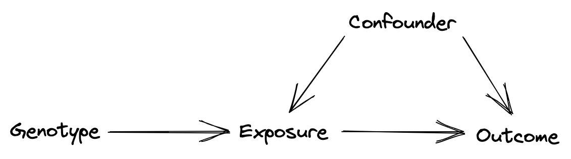
If you want to download the image above to upload into excalidraw, please download it as a png or svg.
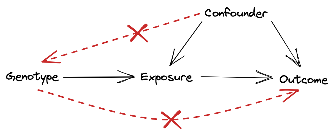
And the DAG showing effects that are not allowed under the IV core conditions.
Session information for reproducibility
Click here for session info
sessionInfo()
#> R version 4.5.3 (2026-03-11)
#> Platform: aarch64-apple-darwin20
#> Running under: macOS Tahoe 26.4.1
#>
#> Matrix products: default
#> BLAS:   /Library/Frameworks/R.framework/Versions/4.5-arm64/Resources/lib/libRblas.0.dylib
#> LAPACK: /Library/Frameworks/R.framework/Versions/4.5-arm64/Resources/lib/libRlapack.dylib;  LAPACK version 3.12.1
#>
#> locale:
#> [1] en_US.UTF-8/en_US.UTF-8/en_US.UTF-8/C/en_US.UTF-8/en_US.UTF-8
#>
#> time zone: Europe/London
#> tzcode source: internal
#>
#> attached base packages:
#> [1] stats     graphics  grDevices datasets  utils     methods   base
#>
#> other attached packages:
#>  [1] DiagrammeR_1.0.11   quickdag_0.2.1.9000 ggdag_0.2.13
#>  [4] dagitty_0.3-4       lubridate_1.9.5     forcats_1.0.1
#>  [7] stringr_1.6.0       dplyr_1.2.1         purrr_1.2.2
#> [10] readr_2.2.0         tidyr_1.3.2         tibble_3.3.1
#> [13] ggplot2_4.0.2       tidyverse_2.0.0
#>
#> loaded via a namespace (and not attached):
#>  [1] gtable_0.3.6       xfun_0.57          htmlwidgets_1.6.4  visNetwork_2.1.4
#>  [5] processx_3.8.7     ggrepel_0.9.8      tzdb_0.5.0         vctrs_0.7.3
#>  [9] tools_4.5.3        generics_0.1.4     curl_7.0.0         pkgconfig_2.0.3
#> [13] RColorBrewer_1.1-3 S7_0.2.1-1         lifecycle_1.0.5    compiler_4.5.3
#> [17] farver_2.1.2       tinytex_0.59       ggforce_0.5.0      graphlayouts_1.2.3
#> [21] codetools_0.2-20   htmltools_0.5.9    yaml_2.3.12        later_1.4.8
#> [25] pillar_1.11.1      MASS_7.3-65        cachem_1.1.0       viridis_0.6.5
#> [29] boot_1.3-32        tidyselect_1.2.1   digest_0.6.39      stringi_1.8.7
#> [33] labeling_0.4.3     quarto_1.5.1       polyclip_1.10-7    fastmap_1.2.0
#> [37] grid_4.5.3         cli_3.6.6          magrittr_2.0.5     ggraph_2.2.2
#> [41] tidygraph_1.3.1    withr_3.0.2        scales_1.4.0       timechange_0.4.0
#> [45] rmarkdown_2.31     igraph_2.2.3       gridExtra_2.3      hms_1.1.4
#> [49] memoise_2.0.1      evaluate_1.0.5     knitr_1.51         V8_8.1.0
#> [53] viridisLite_0.4.3  rlang_1.2.0        Rcpp_1.1.1-1       glue_1.8.1
#> [57] tweenr_2.0.3       renv_1.2.2         rstudioapi_0.18.0  jsonlite_2.0.0
#> [61] R6_2.6.1
quarto::quarto_version()
#> [1] '1.9.37'
tinytex::tlmgr_version()
#> tlmgr revision 78301 (2026-03-07 18:41:28 +0100)
#> tlmgr using installation: /Users/tom/Library/TinyTeX
#> TeX Live (https://tug.org/texlive) version 2026
References
Sanderson, E., G. Davey Smith, F. Windmeijer, and J. Bowden. 2019. “An examination of multivariable Mendelian randomization in the single-sample and two-sample summary data settings.” International Journal of Epidemiology 48 (3): 713–27. https://doi.org/10.1093/ije/dyy262.
Sanderson, E., M. M. Glymour, M. V. Holmes, et al. 2022. “Mendelian randomization.” Nature Reviews Methods Primers 2 (6). https://doi.org/10.1038/s43586-021-00092-5.